1Provincial Meteorological Center of Villa Clara, Cuba.
2Faculty of Health Technology and Nursing (FTSE), University of
Medical Sciences of Villa Clara (UCM-VC), Cuba.
3Specialist in Hygiene and Epidemiology. Assistant Director of Hygiene
and Epidemiology, XX Anniversary Polyclinic. Villa Clara, Cuba.
4Center for Bioactive Chemicals (CBQ), Central University “Marta Abreu”
of Las Villas. Villa Clara, Cuba.
Corresponding author email: rigoberto.fimia66@gmail.com
Article Publishing History
Received: 12/06/2022
Accepted After Revision: 25/08/2022
In this work, 8 meteorological variables were modeled in the Yabú station, Cuba, for which the daily database of this meteorological station was used, where the meteorological variables were taken into account are: extreme temperatures, extreme humidity and its average value, precipitation, wind force and cloudiness corresponding to the period 1977 to 2021. A linear mathematical model was obtained using the Objective Regressive Regression (ORR) methodology for each variable, which explains its behavior according to these variables, 15, 13, 10 and 8 years in advance.
The calculation of the mean error with respect to the persistence forecast in temperatures, wind strength and cloudiness, as well as the persistence model was better with respect to humidity, this allows having valuable long-term information of the weather in a locality, which results in better decision making in the different aspects of the economy and society that are impacted by the weather forecast. It is concluded that these models allow long-term weather forecasting, opening a new possibility for forecasting, so that weather chaos can be overcome if this way of forecasting is used; moreover, it is the first time that an ORR model is applied to weather forecasting processes for a specific day so many years in advance.
Chaos; Forecast; Long Term; Time; Orr Model.
Rodríguez R. O, Duarte R. F, Llanes C. O, González F. M. W. Chaos Theory of Mathematics as seen from a New Perspective for Weather Forecasting. Biosc.Biotech.Res.Comm. 2022;15(2).
Rodríguez R. O, Duarte R. F, Llanes C. O, González F. M. W. Chaos Theory of Mathematics as seen from a New Perspective for Weather Forecasting. Biosc.Biotech.Res.Comm. 2022;15(2). Available from: <a href=”https://bit.ly/3Kzfzuq“>https://bit.ly/3Kzfzuq</a>
Copyright © This is an Open Access Article distributed under the Terms of the Creative Commons Attribution License (CC-BY). https://creativecommons.org/licenses/by/4.0/, which permits unrestricted use distribution and reproduction in any medium, provided the original author and sources are credited.
INTRODUCTION
In different fields of study, cumulative growth models over time play an important role, and many researchers have contributed to the knowledge of the models developed (De Bacco et al., 2018; Dagogo et al., 2020). There are some non-linear models, the most common being Gompertz, Weibull, negative exponential, Richard’s model, logistic, monomolecular, Brody, Mitcherlich, von Betalanffy, S-shaped, among others (Ban, 2020; Dagogo et al., 2020). There are about 77 known equations referred to sigmoidal growth models, which are used in epidemics, bioassays, agriculture, engineering fields, tree diameter, forest height distribution (De Bacco et al., 2018; Dagogo et al., 2020; Wang et al., 2019; Yan et al., 2019). Among the most widely used growth models are those of Gompertz, Richard and Weibull (Ban, 2020; Dagogo et al., 2020). Their formulas can be seen in detail in Ban Ghanim Al-Ani, 2020 (Ban, 2020).
In this research we make a detailed and brilliant mathematical description of them, although the root mean square errors (RMSE) are large for nonlinear models. These models have been implemented in COVID-19, a new disease for which the behavior as time passes; where it was shown for COVID-19 cases in Iraq, that ROR modeling gave better results than nonlinear models, so for meteorology we will use this linear ROR model (Osés et al., 2021a; Osés et al., 2021b).
In this study we develop a linear ROR model of 8 temporal variables, these are: the extreme maximum and minimum temperatures, daily precipitation, maximum and minimum humidity, daily mean, wind strength and cloudiness, which we will compare with the persistence model, which is a good model obtained for weather prediction, and we will show how it is possible to predict it on a given day early enough which shows that the chaos theory can be defeated if this way of prediction is used (Osés et al., 2019; Osés et al., 2021b).
In an article about the Nobel Prize in Physics 2021, it is stated verbatim about mathematical models for weather prediction:”These models are based on the laws of physics and have been developed from models that were used to predict the weather. Weather is described by meteorological quantities such as temperature, precipitation, wind or clouds, and is affected by what happens in the oceans and on land. Climate models are based on the calculated statistical properties of the weather, such as mean values, standard deviations, highest and lowest measured values, and so on. They cannot tell us what the weather will be like in Stockholm on December 10 next year, but we can get an idea of the temperature or the amount of rain we can expect on average in Stockholm in December” *.
This quote evidences the knowledge so far of chaos and its impossibility to go beyond 10 days with the help of predictive weather models, however, according to Brigitte Boisselier, PhD in Physics, Professor of Biochemistry, Director of Clonaid “When a relatively senior, eminent and distinguished scientist declares that something is possible, he or she is probably right. When he agrees that something is impossible, there is a high probability that he is wrong.”
In the case of our research we could not count on the data history of December 10 in Stockholm; however, by having the data from the Yabu weather station (located in the city of Santa Clara, Villa Clara province, Cuba) for that day over the years, and it is with this data that we will demonstrate that long-term weather prediction for this particular day is also possible with an acceptable margin of error, which shows that chaos can be overcome if this way of predicting is used.
MATERIAL AND METHODS
Data from 8 meteorological variables were used (maximum and minimum extreme temperatures, daily precipitation, maximum and minimum humidity, average daily humidity, wind force and cloudiness). The forecast was made using the methodology of Regressive Objective Regression (ROR) which has been implemented in different variables, such as viruses circulating in the province of Villa Clara, population dynamics of culicidae, entomofauna of culicidae and copepods (Sánchez et al., 2017; Fimia et al., 2020a; Fimia et al., 2020b), and particularly in COVID-19 in Cuba (Osés et al., 2021a; Osés et al., 2021c). A long-term forecast was made for up to 15 years, from December 10, 2020 to December 10, 2035.
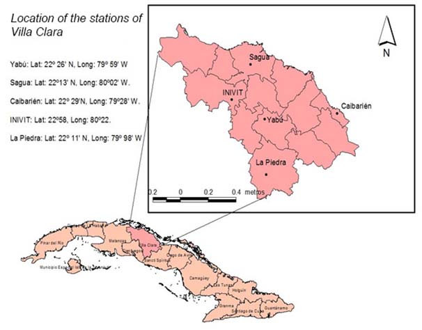
In the linear ROR methodology, first the dichotomous variables DS, DI and NoC must be created, where: NoC: Number of base cases (its coefficient in the model represents the trend of the series). DS = 1, if NoC is odd; DI = 0, if NoC is even, and vice versa. DS represents a saw tooth function and DI this same function, but in inverted form, so that the variable to be modeled is trapped between these parameters and a large amount of variance is explained, a detailed explanation of which can be found in Fimia et al., 2020a. In figure 1 the location of the meteorological stations of Villa Clara province, Cuba.
Figure 1: Geographical distribution of meteorological stations Climate
General description
According to the Köppen classification (modified), in most of Cuba the predominant climate is of the warm tropical type, with a rainy season in the summer. In general, it is quite accepted to express that the climate of Cuba is tropical, seasonally humid, with maritime influence and semi-continental features, our province of Villa Clara also responds to these characteristics. As determining factors in the formation of the climate, the amount of solar radiation received, the particularities of the atmospheric circulation over the country, and the different influence of the physical-geographical characteristics of the territory are identified.
Due to its geographical position, our city is located at a latitude very close to the Tropic of Cancer, which conditions the reception of high values of solar radiation throughout the year, determining the warm character of its climate. In addition, it is located on the border between the zones of tropical and extratropical circulation, receiving the influence of both on a seasonal basis. In the season that goes approximately from November to April, weather and climate variations become more noticeable, with abrupt changes in daily weather, associated with the passage of frontal systems, the anticyclone influence of continental origin and low centers. extratropical pressures.
From May to October, on the contrary, there are few variations over time, with the more or less marked influence of the North Atlantic Anticyclone. The most important changes are related to the presence of disturbances in the tropical circulation (eastern waves and tropical cyclones). All data processing was carried out with the help of the SPSS statistical package, version 19, from IBM. The objective of the work consisted of predicting the long-term meteorological variables at the Yabu weather station, thus defeating the chaos theory.
RESULTS AND DISCUSSION
Table 1 shows the model parameters. The coefficients of the explained variance R are high, the errors of the models are small, the temperatures depend on the lags in 15 years the minimum, and 13 years the maximum, the precipitation in 8 years ago, the minimum humidity in 10 years ago, the wind force (FF) in 13 years and the cloudiness in 15 years ago.
Table 1. Parameters of the models of the different time variables in Yabu, Cuba
| Variables | R | Error of the model | Saw Tooth (DS) | Inverted Saw Tooth (DI) | Tend | Delay
Coeficient |
Fisher F |
| T Min | 98.8 | 3.09 | 10.73 | 8.86 | 15
0.472 |
335 | |
| T max | 99.7 | 2.41 | 51.08 | 49.93 | 13
-0.833 |
1350 | |
| Precip | 100 | 0.0 | -8 E(-16) | -1.5E(-15) | 2.98E(-17) | 8
-5.8E(-17) |
7.51i |
| HRx | 100 | 1.92 | 96.44 | 96.11 | 0.041 | 36861 | |
| Hrn | 98.7 | 9.80 | 77.99 | 73.77 | -0.054 | 10
-0.333 |
277 |
| Hrm | 99.7 | 6.16 | 81.57 | 79.62 | 0.070 | 2490 | |
| FF | 90.2 | 2.91 | 2.353 | 2.586 | 0.049 | 13
0.261 |
27.2 |
| Cloudiness | 92.4 | 1.55 | 2.98 | 2.634 | 15
0.496 |
32.2 |
Table 2 summarizes the linear ROR model obtained by variables, which explains 99.7 % of the variance, with an error of 2.41 ºC, which is a small error considering that we are predicting the maximum daily temperature 13 years in advance.
Table 2. Model summary c,d
| Model | R | R Squaredb | R Squared adjusted | Standar error of estimation | Durbin-Watson |
| 1 | .997a | .993 | .992 | 2.4144 | 2.503 |
- Predictors: Lag13Tmax, DS, DI
- For the regression through the origin (the model without interception), R squared measures the proportion of the variability in the dependent variable on the origin explained by the regression. This CANNOT be compared to R squared for models that include intercept.
- Dependent variable: Tmax
- Linear regression through the origin
Table 3 shows the analysis of variance of the model, which is highly significant with a Fisher’s F of 1350.6 significant at 100 %.
Tabla 3. ANOVA a,b
| Model | Sum os Squares | Df | Cuadratic mean | F | Sig. | |
| 1 | Regressión | 23618.784 | 3 | 7872.928 | 1350.618 | .000c |
| Residuals | 163.216 | 28 | 5.829 | |||
| Total | 23782.000d | 31 | ||||
a. Dependent variable: Tmax
b. Linear regression through the origin
c. Predictors: Lag13Tmax, DS, DI
d. This total sum of squares is not corrected for the constant because the
constant is zero for the regression through the origin.
In table 4, it can be seen that all the variables are significant, the temperature trend is not significant and that is
why it is not shown. The linear model depends on the data returned in 13 years (Lag13 Tmax).
Tabla 4. Coefficient a,b
| Model | Unstandarizaded Coefficient | Standardized Coefficient | t | Sig. | ||
| B | Standard error | Beta | ||||
| 1 | DS | 51.079 | 6.010 | 1.283 | 8.499 | .000 |
| DI | 49.939 | 5.930 | 1.295 | 8.422 | .000 | |
| Lag13Tmax | -.833 | .216 | -.831 | -3.864 | .001 | |
a. Dependent variable: Tmax
b. Linear regression through the origin
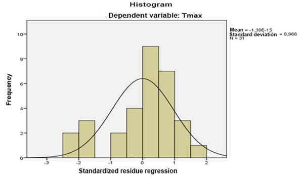
In figure 2 we can see that the residuals do not differ from a normal distribution
with zero mean and 0.966 standard deviation.
Figure 2: Histogram of the standardized residuals for the linear ROR model
In figure 3, the modeling results show that the predicted values coincide with the real values of the variable, where the errors are very small, close to zero.Since no trend was observed in the extreme temperatures, we can affirm that on December 10 throughout history there is no cooling or warming trend, which does not mean that for any other particular day of the daily data series there may be a significant trend.
Figure 3. Maximum Temperature Forecast according to ROR linear model for the Yabu, Cuba meteorological station
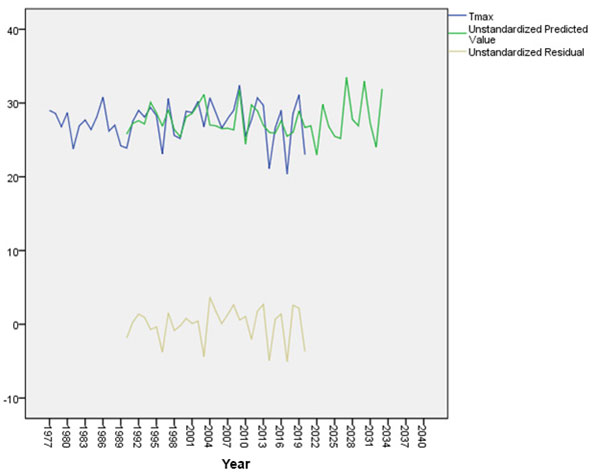
The 13 year ahead forecast is shown in table 5, where it is observed that December 10 will present days with high and lower maximum temperatures. This is the first time that an ROR model is applied to the long-term weather forecast in Cuba 13 years in advance for a specific day, as it had already been done for climatic variables such as sand dumping on Varadero beach with good results (Osés and Pedraza 2021), also for electricity consumption in the province of Villa Clara (Osés et al., 2019); in addition, other works also model the number of people in the long term with cerebrovascular accidents (Osés et al., 2019), as well as the modeling of atmospheric pressure and its impact on the population density of mosquitoes well in advance (Fimia et al., 2020a; Fimia et al., 2020b).
Another long-term model was carried out in Sancti Spiritus, Cuba, where a forecast of daily variables is made one year in advance using ROR regression (Osés et al., 2014), as well as in the prediction of earthquakes (Osés et al., 2018), and of different meteorological disturbances, also of epidemic outbreaks in different geographical latitudes, where global warming of the planet has a high share of responsibility, and where modeling is an essential tool, and even human cloning (Rubin 1978; Wilks 1987; Rael 2001; Rubin 2013; Gelbrecht et al., 2018; Chu et al., 2019; Baker et al., 2020; Reed et al., 2020; Zhang et al., 2020).
Table 5. Case summariesa
| Year | Month | Day | Maximum Temperature (Tmax) | Unstandardized Predicted Value | Unstandardized Residual | ||
| 1 | 1977 | 12 | 10 | 29.0 | . | . | |
| 2 | 1978 | 12 | 10 | 28.6 | . | . | |
| 3 | 1979 | 12 | 10 | 26.8 | . | . | |
| 4 | 1980 | 12 | 10 | 28.7 | . | . | |
| 5 | 1981 | 12 | 10 | 23.8 | . | . | |
| 6 | 1982 | 12 | 10 | 26.9 | . | . | |
| 7 | 1983 | 12 | 10 | 27.7 | . | . | |
| 8 | 1984 | 12 | 10 | 26.4 | . | . | |
| 9 | 1985 | 12 | 10 | 28.2 | . | . | |
| 10 | 1986 | 12 | 10 | 30.8 | . | . | |
| 11 | 1987 | 12 | 10 | 26.2 | . | . | |
| 12 | 1988 | 12 | 10 | 27.0 | . | . | |
| 13 | 1989 | 12 | 10 | 24.2 | . | . | |
| 14 | 1990 | 12 | 10 | 23.9 | 25.77404 | -1.87404 | |
| 15 | 1991 | 12 | 10 | 27.5 | 27.24671 | .25329 | |
| 16 | 1992 | 12 | 10 | 29.0 | 27.60726 | 1.39274 | |
| 17 | 1993 | 12 | 10 | 28.1 | 27.16338 | .93662 | |
| 18 | 1994 | 12 | 10 | 29.4 | 30.10712 | -.70712 | |
| 19 | 1995 | 12 | 10 | 28.3 | 28.66329 | -.36329 | |
| 20 | 1996 | 12 | 10 | 23.1 | 26.85731 | -3.75731 | |
| 21 | 1997 | 12 | 10 | 30.6 | 29.07994 | 1.52006 | |
| 22 | 1998 | 12 | 10 | 25.6 | 26.44067 | -.84067 | |
| 23 | 1999 | 12 | 10 | 25.2 | 25.41348 | -.21348 | |
| 24 | 2000 | 12 | 10 | 28.9 | 28.10724 | .79276 | |
| 25 | 2001 | 12 | 10 | 28.7 | 28.57996 | .12004 | |
| 26 | 2002 | 12 | 10 | 30.2 | 29.77380 | .42620 | |
| 27 | 2003 | 12 | 10 | 26.8 | 31.16315 | -4.36315 | |
| 28 | 2004 | 12 | 10 | 30.7 | 27.02397 | 3.67603 | |
| 29 | 2005 | 12 | 10 | 28.7 | 26.91340 | 1.78660 | |
| 30 | 2006 | 12 | 10 | 26.6 | 26.52399 | .07601 | |
| 31 | 2007 | 12 | 10 | 27.9 | 26.58008 | 1.31992 | |
| 32 | 2008 | 12 | 10 | 29.0 | 26.35734 | 2.64266 | |
| 33 | 2009 | 12 | 10 | 32.4 | 31.82978 | .57022 | |
| 34 | 2010 | 12 | 10 | 25.5 | 24.44078 | 1.05922 | |
| 35 | 2011 | 12 | 10 | 27.7 | 29.74656 | -2.04656 | |
| 36 | 2012 | 12 | 10 | 30.7 | 28.94052 | 1.75948 | |
| 37 | 2013 | 12 | 10 | 29.7 | 26.99672 | 2.70328 | |
| 38 | 2014 | 12 | 10 | 21.1 | 26.02402 | -4.92402 | |
| 39 | 2015 | 12 | 10 | 26.6 | 25.91345 | .68655 | |
| 40 | 2016 | 12 | 10 | 29.0 | 27.60726 | 1.39274 | |
| 41 | 2017 | 12 | 10 | 20.4 | 25.49681 | -5.09681 | |
| 42 | 2018 | 12 | 10 | 28.6 | 26.02402 | 2.57598 | |
| 43 | 2019 | 12 | 10 | 31.1 | 28.91328 | 2.18672 | |
| 44 | 2020 | 12 | 10 | 23.0 | 26.69065 | -3.69065 | |
| 45 | 2021 | 12 | 10 | . | 26.91340 | . | |
| 46 | 2022 | 12 | 10 | . | 22.94087 | . | |
| 47 | 2023 | 12 | 10 | . | 29.82989 | . | |
| 48 | 2024 | 12 | 10 | . | 26.85731 | . | |
| 49 | 2025 | 12 | 10 | . | 25.49681 | . | |
| 50 | 2026 | 12 | 10 | . | 25.19074 | . | |
| 51 | 2027 | 12 | 10 | . | 33.49634 | . | |
| 52 | 2028 | 12 | 10 | . | 27.77392 | . | |
| 53 | 2029 | 12 | 10 | . | 26.91340 | . | |
| 54 | 2030 | 12 | 10 | . | 32.94029 | . | |
| 55 | 2031 | 12 | 10 | . | 27.24671 | . | |
| 56 | 2032 | 12 | 10 | . | 24.02414 | . | |
| 57 | 2033 | 12 | 10 | . | 31.91310 | . | |
| 58 | 2034 | 12 | 10 | . | . | . | |
| 59 | 2035 | 12 | 10 | . | . | . | |
| 60 | 2036 | 12 | 10 | . | . | . | |
| 61 | 2037 | 12 | 10 | . | . | . | |
| 62 | 2038 | 12 | 10 | . | . | . | |
| 63 | 2039 | 12 | 10 | . | . | . | |
| 64 | 2040 | 12 | 10 | . | . | . | |
| Total | N | 64 | 64 | 64 | 44 | 44 | 31 |
a. Limitado a los primeros 100 casos.
Table 6 shows the results of the errors taking an independent sample of 11 cases from 2010 to 2021 to see how the model performs in an independent sample of 25 % of the cases. As can be seen, the errors are small for all variables, as are the standard deviations of the variables.
Mean errors of the time variables for an independent sample of 11 cases, starting in 2010 (Table 6).
Table 6. Descriptive statistics
| N | Minimum | Maximum | Media | Standard desviation | |
| eTmin.mi | 11 | -7.82 | 3.89 | -1.1261 | 4.12549 |
| eTmax.mi | 11 | -5.10 | 2.70 | -.3086 | 3.03874 |
| er24h.mi | 11 | .00 | .00 | .0000 | .00000 |
| eFFmed.mi | 11 | -4.23 | 4.83 | .1066 | 2.84084 |
| eHrmax.mi | 11 | -4.65 | 2.51 | -.1206 | 1.92130 |
| eHrmin.mi | 11 | -8.74 | 12.10 | .5386 | 7.09060 |
| eHrmed.mi | 11 | -8.28 | 6.97 | .3082 | 5.00155 |
| eNmed.mi | 10 | -1.87 | 1.81 | -.1527 | 1.34801 |
| N valid (by list) | 10 |
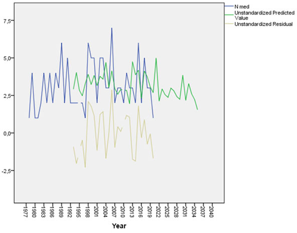
The forecast results for the rest of the meteorological variables in Yabu, Cuba are shown below (Figures 4-10).
Figure 4. Extreme minimum temperature
Figure 5. Daily Precipitation
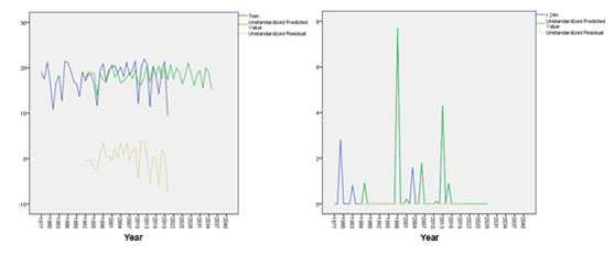
Figure 6. Daily wind force
Figure 7. Maximum daily relative humidity
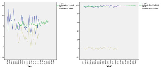
Figure 8. Minimum Relative Humidity
Figure 9. Mean relative humidity
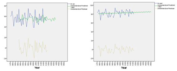
Figure 10. Daily cloudiness on December 10 in Yabu, Cuba
Finally, the improvement index of one model over another was calculated as follows, which is nothing more than the modeling SKILL. Here a slight modification was made to the formula (Wilks 1987) by adding the mean instead of the mean squared error (MSE) according to the original formula, obtaining that the established model is the persistence model and the model to be checked is the ROR, this was done in the independent sample of 11 cases.
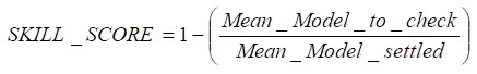
Table 7. Results of mean error in an independent sample of 11 cases
| Variable | Error ROR | Error Persistency | Improvment (%) |
| Temperature Minimum (T Min). | -1.1261 | -1.3175 | 14.5 |
| Temperature Máximum (T max) | -0.3086 | -0.7757 | 60.2 |
| Precipitation | 0.000 | 0.000 | – |
| Maximum Relative Humidity (HRx) | -0.1206 | -0.1105 | * |
| Mínimum Relative Humidity (Hrn) | 0.5386 | 0.5250 | * |
| Mean Relative Humidity (Hrm) | 0.3082 | 0.2002 | * |
| Mean velocity of wind (FF) | 0.1066 | 0.1786 | 40.31 |
| Cloudiness | -0.1527 | -0.3736 | 59.12 |
The improvement ranges from 14.5 % in the minimum temperature to 60.2 % in the maximum, so we can affirm that in this case a linear ROR model exceeds a persistence model in most of the variables studied, except for humidities where persistence exceeds to the ROR model by a narrow margin.
CONCLUSION
The coefficients of the explained variance R were high, while the errors of the models small, where temperatures depended on lags in 15 years, for the minimum and 13 years the maximum; precipitation in 8 years, minimum humidity in 10 years, wind force (FF) in 13 years and cloudiness in 15 years, showing that it is possible to predict well in advance what is going to happen in a day. In the independent sample of 11 years, the errors were small for all variables, as well as the standard deviations of the variables. So we can affirm in this case, that a linear ROR model outperforms a persistence model in most of the variables studied, except for humidities, where persistence outperformed the ROR model by a narrow margin, thus overcoming the chaos in weather forecasting, all of which is very positive, for being the first time that a ROR model is applied to weather forecasting processes for a specific day 8, 10, 13 and 15 years in advance.
ACKNOWLEDGEMENTS
We would like to thank the Villa Clara Cuba Provincial Meteorological Center for providing the computing resources without which this work would not have been possible, as well as Arch. Odalys D. Llanes Concepción for editing the document.
REFERENCES
Baker, R.E., Yang, W., Vecchi, G.A., Metcalf, C.J.E., Grenfell, B.T. (2020). Susceptible supply limits the role of climate in the early SARS-CoV-2 pandemic. Science 369: 315-319.
Ban, G.A. (2021). Statistical modeling of the novel COVID-19 epidemic in Iraq. Epidemiol. Methods 10, 20200025.
Chu, J.E., Timmermann, A., Lee, J.Y. (2019). North American April tornado occurrences linked to global sea surface temperature anomalies. Science Advances 5: eaax0220.
Dagogo, J., Nduka, E.C., Ogoke, U.P. (2020). Comparative Analysis of Richards’, Gompertz and Weibull Models. IOSR Journal of Mathematics 16: 15-20.
De Bacco, C., Larremore, D.B., Moore, C. (2018). A physical model for efficient ranking in networks. Science Advances 4: eaar8260.
Fimia, D.R., Osés, R.R., Alarcón-Elbal, P.M., Aldaz-Cárdenas, J.W., Roig-Boffill, B.V., de la Fé-Rodríguez, P.Y. (2020b). Modelación matemática del efecto de la presión atmosférica sobre la densidad poblacional de los mosquitos (Diptera: Culicidae) en Villa Clara, Cuba. Revista de la Facultad de Medicina 68: 541-549.
Fimia, D.R., Osés, R.R., González, G.R., Hernández, C.N., Otero, M.M. (2020a). La entomofauna de culícidos y los copépodos abordados desde las alternativas de control biológico hasta la modelación matemática en dos provincias centrales de Cuba. Anales de la Academia de Ciencias de Cuba 10: 1-11.
Gelbrecht, M., Boers, M., Kurths, N. (2018). Phase coherence between precipitation in South America and Rossby waves. Science Advances 4: 1-9.
Nobel Prize For Physics (2021) The Royal Swedish Academy Of Sciences Www.Kva.Se Science Editors: Ulf Danielsson, Thors Hans Hansson, Gunnar Ingelman, Anders Irbäck, John Wettlaufer, the Nobel Committee for Physics Text: Joanna Rose Translator: Clare Barnes Illustrations: ©Johan Jarnestad/The Royal Swedish Academy of Sciences Editor: Sara Gustavsson ©Royal Swedish Academy of Sciences
Osés, L.C., Osés, R.R., Fimia, D.R., Zambrano, G.M.P., Wilford, G.F.M. (2021a) Comparison of lineal ROR vs Nonlinear Weibull model for COVID-19 in Iraq. Himalayan Journal of Applied Medical Sciences and Research 2: 88-96.
Osés, R.R., Alonso, F.J.L., Fimia, D.R., Osés, L.C., Burgos, A.I., De La Paz, G.E., Pedraza, M.A., Basanta, M.L.M. (2019). Modelation of the Quantity of Deceaseds and Revenues for Stroke in Sagua La Grande, Villa Clara, Cuba. Impact of the Climate. The Biologist (Lima) 17 (Suplemento Especial 2).
Osés, R.R., Carmenate, R.A., Pedraza, M.A.F., Fimia, D.R. (2018). Prediction of latitude and longitude of earthquakes at global level using the Regressive Objective Regression method. Advances in Theoretical & Computational Physics (Adv Theo Comp Phy) 1: 1-5.
Osés, R.R., Fimia, D.R., Osés, L.C., Zambrano, G.M.P., Santos, Z.T.B., González, M.A. (2021c). Forecast of New and Deceased Cases of COVID-19 in Cuba with an Advance of 105 Days. Acta Scientific Veterinary Sciences 3: 31-36.
Osés, R.R., Fimia, D.R., Saura, G.G., Pedraza, M.A., Ruiz, C.N., Socarras, P.J. (2014). Long Term Forecast of Meteorological Variables in Sancti Spiritus, Cuba. Applied Ecology and Environmental Sciences 2: 37-42 (2014).
Osés, R.R., Machado, F.H., González, M.A.A., Fimia, D.R. (2019). Estudio del consumo eléctrico provincial de Villa Clara y su pronóstico 2019-2023 en Cuba. Revista ECOSOLAR 65: 32-43. URL: http://www.cubasolar.cu/biblioteca/ecosolar
Osés, R.R., Osés, C.L., Fimia, D.R., González, M.A., Iannacone, J., Bruna, S.T., Wilford, G.F.M. (2021b). Age Prediction for COVID-19 Suspects and Contacts in Villa Clara Province, Cuba. EC Veterinary Science 6: 41-51.
Osés, R.R., Pedraza, M.A. (2021). Mathematical Modeling and Forecast 11 Years in Advance of the Dumping of Sand in Varadero Beach, Cuba, Using the Regressive Objective Regression (ROR) Methodology. Journal of Engineering and Applied Sciences Technology 3: 1-3.
Rael, V.C. (2001). Si a la clonación humana. La vida eterna gracias a la Ciencia. NOVA distribution Corporation. Post-Office Box 225, 1211 Ginebra 8- Suiza.www.rael.org.
Reed, K.A., Stansfield, A.M., Wehner, M.F., Zarzycki, C.M. (2020). Forecasted attribution of the human influence on Hurricane Florence. Science Advances 6: eaaw9253.
Rubin, D.B. (1978). Bayesian inference for causal effects: The role of randomization. Ann. Stat 6: 34-58.
Rubin, D.B. (2013). Bayesian Data Analysis (Chapman and Hall/CRC Texts in Statistical Science, ed. 3.
Sánchez, Á.M.L., Osés, R.R., Fimia, D.R., Gascón, R.B.C., Iannacone, J., Zaita, F.Y. (2017). La Regresión Objetiva Regresiva más allá de un ruido blanco para los virus que circulan en la provincia Villa Clara, Cuba. The Biologist (Lima) 15 (Suplemento Especial 1).
Wang, B., Chen, G., Liu, F. (2019). Diversity of the Madden-Julian Oscillation. Science Advances 5: eaax0220.
Wilks, S.D. (1987). Statistical Methods in the Atmospheric Sciences. An introduction. Internacional Geophysics Series 59: 255-256.
Yan, Z., Wu, B., Li, T., Collin, M., Clark, R., Zhou, T., Murphy, J., Tan, G. (2019). Eastward shift and extension of ENSO-induced tropical precipitation anomalies under global warming. Science Advances 6: eaax4177.
Zhang, G., Murakami, H., Knutson, T.R., Mizuta, R., Yoshida, K. (2020). Tropical cyclone motion in a changing climate. Science Advances 6: eaaz7610.