1Department of Computer Science, Faculty of Computing and Information technology, King Abdulaziz University, Jeddah, Saudi Arabia
2Deanship of Information Technology, King Abdulaziz University, Jeddah, Saudi Arabia
Corresponding author Email: waljedaibi@kau.edu.sa
Article Publishing History
Received: 03/11/2018
Accepted After Revision: 19/12/2018
Successful implementation of large-scale software systems urgently needs to apply Critical Success Factors “CSF”. Data accuracy is one of the important CSFs which need to be measured and monitored carefully during the implementation of LSSs. This article focused on developing a method for measuring, monitoring and controlling Critical Success Factors of large scale software systems called “CSF- Live”. Then, we apply CSF-Live for the data accuracy CSF. The CSF-Live uses the Goal/Question/Metric paradigm (GQM) to yield a flexible framework contains several metrics that we used to develop a formulation which enables the measurement of the data accuracy CSF. The formulation that we developed it for the data accuracy CSF is crucial to maintain accurate data in the legacy system during the transformation to the LSS.
Enterprise Resource Planning Systems (Erps), Critical Success Factors (Csf), Measurement, Goal/Question/Metric Paradigm (Gqm), Data Accuracy
Aljedaibi W, Khamis S. On the Measurement of Data Accuracy During Large-Scale Software Systems Implementations. Biosc.Biotech.Res.Comm. VOL 12 NO1 (Spl Issue February) 2019.
Aljedaibi W, Khamis S. On the Measurement of Data Accuracy During Large-Scale Software Systems Implementations. Biosc.Biotech.Res.Comm. VOL 12 NO1 (Spl Issue February) 2019. Available from: https://bit.ly/2XwSXWo
Introduction
Large-scale software systems (LSS) represented by Enterprise Resource Planning systems (ERPs) are complex according to its great size as well as the number of applications and services that they offer it. These systems work in different environments in which influential factors exist, termed as Critical Success Factors (CSFs). Data accuracy is among the CSFs and refers to either the data values stored for an object are the correct values or not, i.e. which means that data values must be represented in a consistent and unambiguous form; for example, if the following date September 20, 1959 is to be expressed in USA format then the it should be displayed as 9/20/1959.” [16]. Large-scale software systems are complex, and they need to have precise data to work effectively. So, the data must be true and accurate when used in ERP systems to ensure no disruption to performance and it is working efficiently and with fewer errors [17].
Inaccurate data negatively affect the functioning of system’s modules. If there are errors in data such as empty mandatory fields, then developers must monitor this data or try to alter them in the early stage before large-scale software system is implemented [4]. During the implementation of new ERP systems, we suggest that usage of legacy systems should continue but with no further development and enhancement, however, we measure and monitor the data accuracy in legacy system during transformation from legacy system to the large-scale software systems. we need to make sure that data accuracy does not decline and no any radical changes during the new project implementation. Despite the importance of data accuracy, there were no attempts to measure it using numerical values. However, it was measured using descriptive measures, e.g. high, medium and low [18]. In this work, we changed this descriptive method by proposing a new method to quantify the data accuracy factor. Using this quantified measure, we can monitor data accuracy in a more accurate manner. The proposed method is based on the GQM paradigm.
This article has the following sections: in Section 2 presents a background, while paper design and methodology is discussed in Section 3. Section 4 shows CSF-Live Method then Section 5 shows Measure of Data Accuracy. Conclusion are presented in Section 6.
Background
The difficulty to manage and implement Large-scale software systems (LSS) is raised from different aspects related to the project management, requirement analysis, design, implementation, testing the LSS, and post-implementation maintenance [1]. These steps requires careful attention and detailed execution by experienced team. ERP is a common examples of LSS [4]. An ERP can be defined as a software concerned in business management which is implemented and effectively used by a company collect, store, manage, and interpret data that is obtained from many business activities including human resource, administrative, customer service, financial management, production, sales, business intelligence and functional in corporations and organizations, as shown in Figure 2.1 [9].
![Figure 2.1. ERP various Modules [9]](http://bbrc.in/wp-content/uploads/2020/11/fig2.1_opt.jpeg) |
Figure 2.1: ERP various Modules [9] |
Numerous studies and research discussed [4, 10, 11] several ERP implementations have failed or encountered serious delays. Many issues and obstacles appeared in the performance of these tasks within the ERPs [12]. It was noticed that during such projects there were several factors that yielded such final results and that gave rise to what is known today as the critical success factors (CSFs) of large-scale software systems [4].
There are above 66 critical success factors that have been reported [4], and which were found to affect ERP implementations. These factors have been further reduced to 18 factors as shown in Figure 2.2.
![Figure 2.2. Set of Critical Success Factors [4]](http://bbrc.in/wp-content/uploads/2020/11/fig2.2_fmt.jpeg) |
Figure 2.2: Set of Critical Success Factors [4] |
There were no previous attempts to measure these factors which we believe is important to assess the status of each and its subsequent impact on the success or failure of the program. Basili et al. introduced the Goal/Question/Metric paradigm (GQM) to address measurement of some goal, which maybe an object as well, according to the following approach:
- Identification of (a) goal(s) of the project.
- Ask questions related to how the goal can be achieved.
- Identify metrics.
GQM consists of three levels [8]:
- Conceptual level (Goal)
We define a goal for a specific object in a particular environment, using different quality models and for a variety of reasons from different points of view.
- Operational level (Question)
It is the use of a group of questions to determine the project goal and identify the evaluation characteristics or complete a specific goal.
- Quantitative level (Metric)
A group of metrics, based on the models, are associated with each question in order to answer it in a measurable manner.
The Goals is the top of GQM model and it is refined to many questions. Answers of these questions called “metrics”. The same metric can be the answer for more than one question as shown in Figure 2.3. Differing viewpoints in answering some of the questions affect the determination of the metrics.
 |
Figure 2.3: GQM Model Hierarchical Structure |
Basili et.al. described his GQM process composed of six steps as in follows [8]:
- Establish a set of goals and objectives for the project associated with the measurement of productivity and quality.
- Ask questions to define those goals clearly.
- Determine measurements to be collected, which will help you get answers.
- Develop data collection methods.
- Collect and validate data on time.
- Collect and validate data on time.
Measurement goals have to be defined in an understandable manner and should be clearly structured [14]. The goal is defined by filling in a set of values for the several parameters in the template, it includes purpose (what object and why), perspective (what aspect and who) and the characteristics of the environment (where) see more Table 2.1.
| Table 2.1: GQM Goal Definition Template [8] | |
| The object under measurement (process, product, other experience models). | Analysis |
| Characterization, evaluation, prediction, motivation, improvement, understanding, controlling, or improving the object. | For the purpose of (Why) |
| The quality focus of the object that the measurement focuses on (cost, correctness, defect removal, change, reliability and user friendliness….). | With respect to |
| The people that measure the object (user, customer, manager, developer and corporation….). | From the viewpoint of
(Who) |
| The environment in which measurement tasks place (problem factors, people factors, resource factors and process factors….). | In the context of |
Paper Design & Methodology
To achieve the goals of this article, the following steps were followed which were applied on data accuracy factor:-
- Study of critical success factors for large-scale software systems
We present a study of the previous research that focus on the critical success factors for implementing large scale software systems (e.g. ERP systems) and from which we selected data accuracy factor of these factors to be studied in the framework
- Apply GQM-analysis
To measure the impact of the data accuracy to the success/failure of the project of implementing large-scale software system, we used GQM to reach a set of metrics directly linked to data accuracy factor to enable monitoring and controlling capabilities.
- Measurement Formulation
Using GQM analysis, a formulation of the metric is presented as part of the measurement model for data accuracy factor.
Csf-Live Method
In this work we used a method (CSF-Live) [15] that represent our proposed framework for measuring data accuracy factor. The purpose of the CSF-Live method is to measure, track, monitor, and control the critical success factors during the implementation of large-scale software systems by using the Goal/Question/Metric (GQM) paradigm. The CSF-live method has six steps as shown in Figure 4.1.
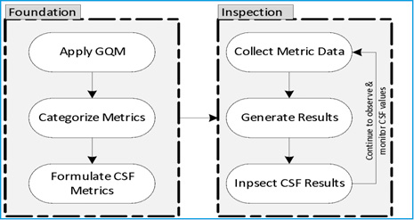 |
Figure 4.1: CSF-Live! Method |
Measure of Data Accuracy
5.1 Data Accuracy as a Numeric Value
Despite the importance of data accuracy, there were no attempts to measure it using numerical values. However, it was measured using descriptive measures, e.g. high, medium and low [18]. In this work, we changed this descriptive method by proposing a new method to quantify the data accuracy factor. Using this quantified measure, we can monitor data accuracy in a more accurate manner. The proposed method is based on the GQM paradigm.
As shown in Table 5.1, a goal has been formulated to measure data accuracy and from the workshop that we conducted with the graduate students and some staff at King Abdulaziz University (KAU), we generated a set of questions and metrics during the discussion which helped us to measure the goal. The generation of questions and metrics is driven by the actual formulation of the goal. In addition, metrics must be represented numerically so that we can quantify the performance of the goal.
| Table 5.1: GQM for Data Accuracy |
| Goal |
| Analyzing the data accuracy in order to achieve the purpose of evaluation with respect to data precision/data correction in view point of project manager/project sponsor in context of legacy software system. |
| Questions |
| How many tables?
Is there new data stored in tables? How many columns in all tables? How many empty cells? Is there new data stored in lookup tables? How many empty mandatory fields? Is there duplicated data between tables? How many scripts run on data? How many batches requests? |
| Metrics (Answers) |
| # Tables
# Records # Columns DB Size # Empty Cells/Table # Lookup Tables Records # Empty Mandatory Fields # Duplicated Records # Batches |
A formulation of the derived metrics will yield a single number that represents the goal, through which progression towards goal achievement can be monitored. It should be noted, that our method to CSF measurement does shows an accurate indication of current status of a single CSF quantified numerically. Figure 5.1 depicts the GQM analysis for data accuracy (top-down) where level one (top) represents the goal and level two (middle) represents questions and level three (down) contains the metrics. Sometimes, the same question is associated to more than one metric. For example, the question “Is there new data stored in tables?” is associated with two metrics “Number of Records” and “Size of DB”. As mentioned earlier, for data collection we created a batch of queries to read from the HR active database daily for 189 days.
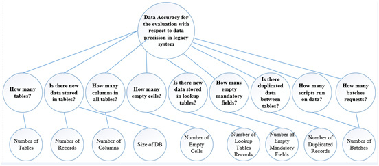 |
Figure 5.1: GQM Analysis for Data Accuracy |
In order to measure the data accuracy, we created a collect resource system (HR) at an enterprise level organization joining more than 9,000 employees. In this case, 130 tables from which our scripts collected 189 days are putted on our database. It is presumed that any change in values of metrics above indicates a possible change in data. In general, change in data is not prohibited but data changes in legacy systems are expected to be less sensitive to ERP requirements of new standards of data structuring. Consequently, if any metric in the legacy system database is increasing while we implement the new ERP system for example, then this signals a risk that may affect accuracy of the data stored in the database. For example, when analyzing data collected for number of records metrics, we noticed that 872,190 new records were added in the HR database through 189 days. Such great increases in the number of records increases the probability of errors such as adding empty mandatory fields etc. This data represents 27 weeks in which the value of metrics was collected in two weeks interval and every two weeks, it is accumulated for a period of 27 weeks. Then, we calculated the following metrics’:-
- Maximum values of metric during the measured time interval.
- Minimum values of metric during the measured time interval.
- Stability Ratio is calculated by minimum values of metric divided by maximum values of metric.
- Metric Change Ratio which is calculated as (1-Stability Ratio).
Metric Change Ratio yields results between zero and one as shown in Figure 5.2. Metric Change Ratio of 1 (or close to 1) means that a number of new changes have been added to the database. On the other hand, Metric Change Ratio of 0 (or close to 0) means that no new (few) changes have been added to the database. We confirm and assure that adding new data to a legacy system database will not be a recommended practice and may lead to a decline in the total accuracy of the data as will be shown later on in next paragraphs. Table 5.2 illustrates us the interpretation of different values for Metric Change Ratio for the new data. The following sections explain the details of each metric related to data accuracy.
 |
Figure 5.2: Bounds of Metric Change Ratio |
| Table 5.2: Interpretation of Metric Change Ratio | |
| Metric Change Ratio | Meaning |
| 0 | 0% New Data |
| 0.01 | 1% New Data |
| 0.02 | 2% New Data |
| 0.03 | 3% New Data |
| 0.04 | 4% New Data |
| 0.05 | 5% New Data |
| 0.06 | 6% New Data |
| …… | …… |
| …… | …… |
| 0.99 | 99% New Data |
| 1 | 100% New Data (Impossible) |
Number of Tables Metric
The number of tables metric is defined as: a numerical count of the data tables within a single database of a legacy system. Figure 5.3 shows the actual data that we obtained representing the number of tables metric which were read from HR database. No changes were observed during the first six weeks, after which six more additional tables were added to the database within 12 weeks. Subsequently, Number of Tables Change Ratio was increased. Then, the number of tables was stable during the last 9 weeks as shown in Figure 5.3. We noticed that increasing the number of tables lead to an increase in the number of columns and number of records which have a negative impact on the data accuracy in the legacy system.
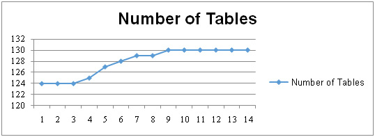 |
Figure 5.3: The Change in the Number of Tables |
Number Of Records Metric
The number of records metrics is defined as: a numerical count of the data records within a single database of a legacy system. Figure 5.4 shows the actual data that is obtained representing the number of records metrics which we were read from HR database. We note that records were continuously increasing since the beginning of the first week until the last week as shown in Figure 5.4, thus increased the Number of Records Change Ratio.
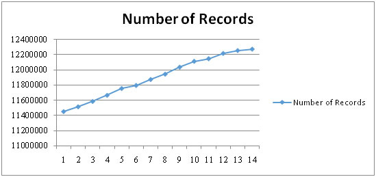 |
Figure 5.4: The Change in the Number of Records |
The Number Of Columns Metric
The number of columns metric is defined as: a numerical count of the data columns within a single database of a legacy system. Figure 5.5 shows the actual data that is obtained representing the number of columns metric which we were read from HR database. We note strong relationship between the increase in the number of tables and increase the number of columns as in the eighth week created one table and two columns and in the tenth week created two tables and twelve columns.
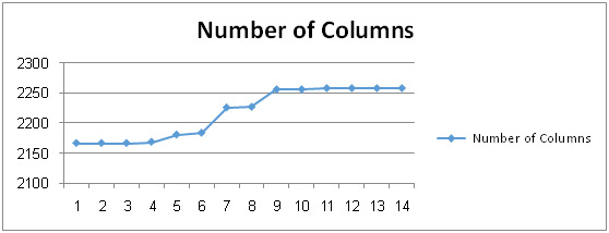 |
Figure 5.5: The Change in the Number of Columns |
Table 5.3 shows detailed comparison between the increase in the number of tables and columns during the project. Sometimes columns are added onto existing tables without creating new tables as in the sixteenth week where one column was added while the number tables were fixed. Also, in the 22nd week, two columns were created while the number tables did not change; but this introduced a new weakness to data accuracy since the number of empty cells in all of the older records within the database is increased. To be accurate, this column addition introduced empty fields in that are equal in count to the number of all older recorded existed in the table. A negative impact on the data accuracy in the legacy system because of the increase in the number empty cells on the pervious data (i.e. the previous records that already exist in the tables). We note that columns were stable during the first six weeks but after that 91 columns were created in the database in the next 16 weeks and thus increased the Number of Columns Change Ratio. Then, the number of columns was stable during the last 5 weeks (i.e. from the 23rd week until the 27th week) as shown in Figure 5.5.
| Table 5.3: Comparison between Number of Tables and Columns | |||
| Sequence | Weeks | Tables | Columns |
| 1 | 1-2 | 0 | 0 |
| 2 | 1-4 | 0 | 0 |
| 3 | 1-6 | 0 | 0 |
| 4 | 1-8 | 1 | 2 |
| 5 | 1-10 | 2 | 12 |
| 6 | 1-12 | 1 | 3 |
| 7 | 1-14 | 1 | 42 |
| 8 | 1-16 | 0 | 1 |
| 9 | 1-18 | 1 | 29 |
| 10 | 1-20 | 0 | 0 |
| 11 | 1-22 | 0 | 2 |
| 12 | 1-24 | 0 | 0 |
| 13 | 1-26 | 0 | 0 |
| 14 | 1-27 | 0 | 0 |
Size Of Database (Db) Metric
The size of database (DB) metric is defined as: a numerical count of the size of database of a legacy system. Figure 5.6 shows the actual data that is obtained representing the size of database metric which we were read from HR database. We measure the size of database in KB. It is highly correlated with the number of records in the database, such that the more number of records the more increase in the database size. We note that the size of the database was stable during the first few weeks but after that increased size of database because number of records was increased and consequently the number block to store this data in the database increased. We notice that the Size of Database Change Ratio was small. In the last few weeks, the size of database did not change as shown in Figure 5.6.
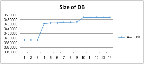 |
Figure 5.6: The Change in the Size of DB |
Number Of Empty Cells Metric
The number of empty cells metric is defined as: a numerical count of the data empty cells within a single database of a legacy system. The empty cells appear when users insert data records into the tables and leave some fields empty or maybe the empty cells are created by running a specific batch. This empty cell issue happens when the database designer allows the crated column(s) to be empty (ability to have NULL value). Figure 5.7 shows the actual data that is obtained representing the number of empty cells metric which we were read from HR database. We note that empty cells were did not change during all weeks as shown in Figure 5.7 therefore the Number of Empty Cells Change Ratio is zero because of no increase in the number of empty cells. Usually, increasing the number of empty cells occur if the number of records is increasing in the database.
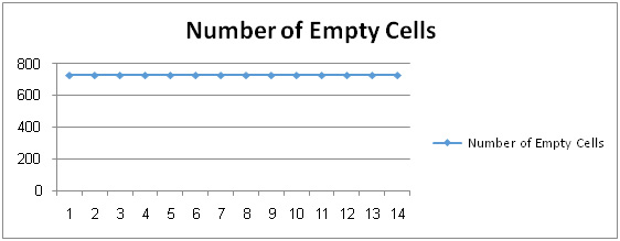 |
Figure 5.7: The Change in the Number of Empty Cells |
Number Of Lookup Tables Records Metric
The number of lookup tables records metric is defined as: a numerical count of the data lookup tables records within a single database of a legacy system. The lookup tables refer to tables that contain static, unchanging information often and that can provide keys usable in other tables [19]. Lookup tables are important in any database. They are used by different queries to connect tables and identify relationship. Figure 5.8 shows the actual data that is obtained representing the number of lookup tables records metric which we were read from HR database. This data consists of 15 weeks only because we needed few weeks’ time to determine lookup tables an identify them in the database. It was shown that the numbers of lookup tables’ records were increasing continuously since the beginning of the fourteenth week until the last week except of the last six weeks as there was no change in the number of lookup tables’ records as shown in Figure 5.8. Also, we note a small increase in the Number of Lookup Tables Records Change Ratio because of limited number of inserted lookup tables’ records.
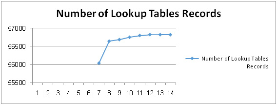 |
Figure 5.8: The Change in the Number of Lookup Tables Records |
5.8 Number Of Empty Mandatory Fields Metric
The number of empty mandatory fields metric is defined as: a numerical count of the data empty mandatory fields within a single database of a legacy system. The mandatory fields refer to fields that must be filled when user insert data to the table. Empty mandatory fields appear when designer allows the column to be empty when he creates the column. Mandatory fields are also called “required” fields. Figure 5.9 shows the actual data that is obtained representing the number of empty mandatory fields metric which we were read from HR database. We note that empty mandatory fields were zero during all weeks as shown in Figure 5.9; this means that either designer did not allow the mandatory fields to be empty or users entered data in the all the mandatory fields as part of application requirement. Therefore, Number of Empty Mandatory Fields Change Ratio was zero because of no increase in the number of empty mandatory fields.
| Table 5.4: Measurement of the Data Accuracy | |||||||||||
| Sequence | Weeks | Number of Tables Change Ratio | Number of Records Change Ratio | Number of Columns Change Ratio | Size of Database Change Ratio | Number of Empty Cells Change Ratio | Number of Lookup Tables Records Change Ratio | Number of Empty Mandatory Fields Change Ratio | Number of Duplicated Records Change Ratio | Number of Batches Change Ratio | DA |
| 1 | 1-2 | 0 | 0.01 | 0 | 0 | 0 | 0 | 0 | 0 | 0.9 | 0.91 |
| 2 | 1-4 | 0 | 0.01 | 0 | 0 | 0 | 0 | 0 | 0 | 0.9 | 0.91 |
| 3 | 1-6 | 0 | 0.02 | 0 | 0 | 0 | 0 | 0 | 0 | 0.9 | 0.92 |
| 4 | 1-8 | 0.01 | 0.02 | 0 | 0.02 | 0 | 0 | 0 | 0 | 0.9 | 0.95 |
| 5 | 1-10 | 0.02 | 0.03 | 0.01 | 0.02 | 0 | 0 | 0 | 0 | 0.9 | 0.98 |
| 6 | 1-12 | 0.03 | 0.03 | 0.01 | 0.02 | 0 | 0 | 0 | 0 | 0.9 | 0.99 |
| 7 | 1-14 | 0.04 | 0.04 | 0.03 | 0.02 | 0 | 0 | 0 | 0 | 0.9 | 1.03 |
| 8 | 1-16 | 0.04 | 0.05 | 0.03 | 0.02 | 0 | 0.01 | 0 | 0 | 0.9 | 1.05 |
| 9 | 1-18 | 0.05 | 0.05 | 0.04 | 0.02 | 0 | 0.01 | 0 | 0 | 0.9 | 1.07 |
| 10 | 1-20 | 0.05 | 0.06 | 0.04 | 0.03 | 0 | 0.01 | 0 | 0 | 0.9 | 1.09 |
| 11 | 1-22 | 0.05 | 0.06 | 0.04 | 0.03 | 0 | 0.01 | 0 | 0 | 0.9 | 1.09 |
| 12 | 1-24 | 0.05 | 0.07 | 0.04 | 0.03 | 0 | 0.01 | 0 | 0 | 0.9 | 1.1 |
| 13 | 1-26 | 0.05 | 0.07 | 0.04 | 0.03 | 0 | 0.01 | 0 | 0 | 0.9 | 1.1 |
| 14 | 1-27 | 0.05 | 0.07 | 0.04 | 0.03 | 0 | 0.01 | 0 | 0 | 0.9 | 1.1 |
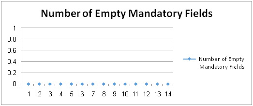 |
Figure 5.9: The Change in the Number of Empty Mandatory Fields |
Number Of Duplicated Records Metric
The number of duplicated records metrics is defined as: a numerical count of the data duplicated records within a single database of a legacy system. The number of duplicated records metrics refers to the number of duplicated the data records in different tables. Figure 5.10 shows the actual data that is obtained representing the number of duplicated records metrics which we were read from HR database. We note that duplicated records are zero during all weeks as shown in Figure 5.10. This means repeating rows data is difficult to be replicated in the tables of the database, yet the duplicated records metric is important to measure data accuracy in legacy system. In HR the Number of Duplicated Records Change Ratio was zero because of no increase in the number of duplicated records.
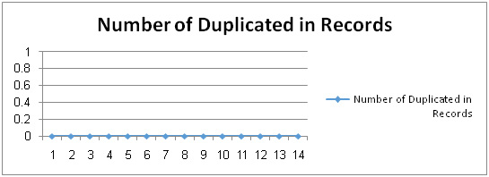 |
Figure 5.10: The Change in the Number of Duplicated in Record |
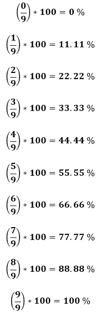
| Table 5.5: Interpretation of Data Accuracy | |
| Result | Meaning |
| 0 | 0% Change |
| 1 | 11.11% Change |
| 2 | 22.22% Change |
| 3 | 33.33% Change |
| 4 | 44.44% Change |
| 5 | 55.55% Change |
| 6 | 66.66% Change |
| 7 | 77.77% Change |
| 8 | 88.88% Change |
| 9 | 100% Change (Impossible) |
Number Of Batches Metric
The number of batches metric is defined as: a numerical count of the data batches within a single database of a legacy system. The number of batches metric refers to the execution of a series of programs on a data without manual intervention (non-interactive) [20]. In HR database, Job Control Language (JCL) is a program that has many batches. During working days there exist 7 Job Control Language which have 70 batches that are executed every day except weekend. During weekends, there exists 3 Job Control Language which have 7 batches to work. In addition, there are some batches that are executed by requests from other departments in the deanship to perform some specific functions on the data. Batches execution has a negative impact on the data accuracy in legacy system because of the risk of creating new data which may have errors or empty.
Figure 5.11 shows the actual data that is obtained representing the number of batches metric which we were read from HR database. We note that there is great difference between maximum batches and minimum batches because many of the batches work only on working days, so Number of Batches Change Ratio is big number and also it is stable during the weeks as shown in Figure 5.11.
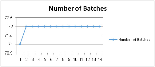 |
Figure 5.11: The Change in the Number of Batches |
Formulation Of Data Accuracy (Da) Metric
We formulated data accuracy as the summation of all the nine ‘change ratio’ metrics that we described in the previous sections as shown in Table 5.4:
DA = TCR + RCR + CCR + SCR + ECCR + LTRCR
+ EMFCR + DRCR + BCR
where
TCR: Number of Tables Change Ratio,
RCR: Number of Records Change Ratio,
CCR: Number of Columns Change Ratio,
SCR: Size of Database Change Ratio,
ECCR: Number of Empty Cells Change Ratio,
LTRCR: Number of Lookup Tables Records Change Ratio,
EMFCR: Number of Empty Mandatory Fields Change Ratio,
DRCR: Number of Duplicated Records Change Ratio,
BCR: Number of Batches Change Ratio.
The actual data is shown in for all nine-change ratio of metrics and values of the data accuracy Table 5.4.
Data accuracy is calculated in two successive weeks then accumulated every two weeks until the 27th week. From the achieved results, we notice that the highest impact on the performance of data accuracy is represented by the Number of Batches Change Ratio while on the other hand the Number of Empty Cells Change Ratio, Number of Empty Mandatory Fields Change Ratio and Number of Duplicated Records Change Ratio did not effect on the performance of data accuracy in this legacy system. In addition to this important note, we observe that in the first four weeks that the data accuracy did not change but after that increased in the next 20 weeks due to the increase in some values of the change ratio metrics but in the last 3 weeks the data accuracy become constant without any change as illustrated in Figure 5.12.
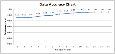 |
Figure 5.12: Measurement of the Data Accuracy |
As shown in Fig. 5.13, Data accuracy gives results ranging from zero to nine. The accuracy of data 9 (or approximately 9) means that a number of new changes have been added to the database. On the other hand, data accuracy (0 or close to 0) means that no new changes have been added to the database. According to that result, we confirm that adding new changes to the old system database is not a recommended practice as it may result in a reduction in the overall accuracy of the data. Accordingly, the percentage of the extent of the accuracy of the data is calculated for each value obtained for the accuracy of the data.
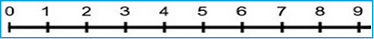 |
Figure 5.13: Bounds of Data Accuracy |
For example, at the end of the 12th week of data collection, the result of data accuracy was: 0.99
This means that the change in the data accuracy was by 11%
![]()
Since:
Our data shows that the value of the data accuracy metric based on 27 weeks of data collection was:
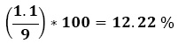
Data Accuracy Metric = 1.1
This means the change in the data accuracy was 12.22%, since:
In a summary, the higher the change percentage the lower the data accuracy becomes. Table 5.5 shows us the summary of interpretation of different data accuracy values and the corresponding change percentage in data accuracy described in the following formula:
Concluded Comments
Large-scale software systems (LSS) are seen as a complex problem given their size, quantity, source lines, number of users, number of data sizes, and the variety of services and applications they provide. In this regard, there are many factors play a major and pivotal role in the successful implementation of LSS, which are called critical success factors (CSFs) for large-scale software systems. In this paper, we chose the CSF to investigate it by measuring its impact on the old software system during the conversion to the software system on a large scale. So, we apply CSF-Live! . This parameter is a way used to measure and control the data accuracy factor that may affect the implementation of programs on a large scale. We have also created a set of metrics that are numerically represented to enable goal control, control and data collection to reflect metrics. Finally, we succeeded in formulating a mathematical expression representing the data accuracy factor, the data collected, and presented a case study that explored and explained the results.
Reference
- Bar, Adnan Al, et al. “An Analysis of the Contracting Process for an ERP system.”, SEAS-2013, Computer Science Conference Proceedings in Computer Science & Information Technology (CS & IT) series, Dubai, UAE, November 2-3, 2013
- She, Wei, and Bhavani Thuraisingham. “Security for enterprise resource planning systems.” Information Systems Security 16.3 (2007): 152-163.
- Oracle Corporation, Redwood Shores, CA 94065 U.S.A, 10 Reasons Why Oracle Infrastructure Provides the Best Platform for SAP Environments April 2012, Version 1.0
- Ahmad Mutahar, “An Empirical Study of Critical Success Factors for ERP Software System Implementations in Saudi Arabia”, Master thesis, Work under progress, 2016.
- Somers, Toni M., and Klara Nelson. “The impact of critical success factors across the stages of enterprise resource planning implementations.” System Sciences, 2001. Proceedings of the 34th Annual Hawaii International Conference on. IEEE, 2001.
- Holland, Christoper P., Ben Light, and Nicola Gibson. “A critical success factors model for enterprise resource planning implementation.” Proceedings of the 7th European Conference on Information Systems. Vol. 1. 1999.
- Boynton, Andrew C., and Robert W. Zmud. “An assessment of critical success factors.” Sloan management review 25.4 (1984): 17.
- Caldiera, Victor R. Basili-Gianluigi, and H. Dieter Rombach. “Goal question metric paradigm.” Encyclopedia of Software Engineering 1 (1994): 528-532
- Bauer, Rich. Just the FACTS101 e-Study Guide for: Introduction to Chemistry. Cram101 Textbook Reviews, 2012.
- Fang, Li, and Sylvia Patrecia. “Critical success factors in ERP implementation.” (2005).
- Allen, David, Thomas Kern, and Mark Havenhand. “ERP Critical Success Factors: an exploration of the contextual factors in public sector institutions.” System Sciences, 2002. HICSS. Proceedings of the 35th Annual Hawaii International Conference on. IEEE, 2002
- Bar, Adnan Al, et al. “An experience-based evaluation process for ERP bids.”, arXiv preprint arXiv:1311.2968 (2013)
- Melia, Detta. “Critical Success Factors and performance Management and measurement: a hospitality context.” (2010)
- Esteves, Jose, Joan Pastor-Collado, and Josep Casanovas. “Monitoring business process redesign in ERP implementation projects.” AMCIS 2002 Proceedings (2002): 125.
- Sufian Khamis and Wajdi Aljedaibi, A Framework for Measuring Critical Success Factors of Large-Scale Software Systems. International Journal of Computer Engineering and Technology, 7(6), 2016, pp. 71–82.
- Olson, Jack E. Data quality: the accuracy dimension. Morgan Kaufmann, 2003.
- Wu, Jun. “Critical success factors for ERP system implementation.” Research and Practical Issues of Enterprise Information Systems II. Springer US, 2007. 739-745.
- Osman, M. R., et al. “ERP systems implementation in Malaysia: the importance of critical success factors.” International Journal of Engineering and Technology 3.1 (2006): 125-131.
- Quamen, Harvey et al. Digital Humanities Database, 2012.
- Furdal, Stanislaw, and N. J. Plainsboro. “Quick Windows Batches to Control SAS® Programs Running Under Windows and UNIX,2008