Department of Computer Science & Engineering, DIT University, Dehradun, India

Corresponding author Email: vaibhav05cse@gmail.com

Article Publishing History

Introduction

Deep learning, a family of machine learning algorithms, is inspired by the biological process of neural networks is dominating in many applications and proving its advantage over conventional machine learning algorithms (Good fellow et al, 2016). It is only because of their capability in producing faster and more accurate results. It attempts to model high-level abstraction in data based on a set of algorithms (Deng et al, 2014). In deep learning techniques, there is a direct learning from the data for all aspects of the model. It starts with lowest level features that present a suitable representation of the data. It then provides higher-level abstractions for each of the specific problem in which it is applied. Deep learning becomes more useful when the amount of training data is increased. The development of deep learning models has increased with the increase in the software and hardware infrastructure (Aghdam et al., 2017, Nisbet et al, 2018).

Deep learning models use multiple layers which are the composition of multiple linear and non-linear transformations. With the increase in the size of data, or with the developments in the field of big data, conventional machine learning techniques have shown their limitation in analysis with the size of data (Chen, 2014). Deep learning techniques have been giving better results in this task of analysis. This technique has been introduced worldwide as breakthrough technology because has differentiated machine learning techniques working on old and traditional algorithms by exploiting more human brain capabilities.It is useful in modeling the complex relationship among data. Instead of working on task-specific algorithms it is based on learning data representations. This learning can be supervised, unsupervised or semi-supervised, (Hoff, 2018).

In deep learning models, multiple layers composed of non-linear processing units perform the task of feature extraction transformation. Every layer takes the input as the output of its corresponding previous layer. It is applied in classification problems in a supervised manner and in pattern analysis problems in an unsupervised manner. The multiple layers which provide the high-level abstraction, form a hierarchy of concepts. There are deep learning models which are mostly based on artificial neural networks which are organized layer-wise in deep generative models. The concept behind this distributed representation is the generation of observed data through the interaction of layered factors. The high-level abstraction is achieved by these layered factors. A different degree of abstraction is achieved by varying the number of layers and the size of layer (Najafabadi et al, 2015).

The abstraction is achieved through learning from the lower level by exploiting the hierarchical exploratory factors. By converting the data into compact immediate representations of principal components and removing redundancies in representation through derived layered structures, the deep learning methods avoid feature engineering in supervised learning applications. In unsupervised learning where unlabeled data is more abundant than labeled data, deep learning algorithms can be applied to such kind of problems. The deep belief networks are the example of deep learning model which are applied to such unsupervised problems, (Auer et al., 2018).

Deep learning algorithms exploit the abstract representation of data which is because of the fact that more abstract repetitions are based on less abstraction. Due to this fact, these models are invariant to the local changes in the input data. This has the advantage in many pattern recognition problems. This invariance helps the deep learning models feature extraction in the data. This abstraction in representation provides these models the ability to separate the different sources of variations in data. The deep learning models outperform old machine learning models by manually defining the learning features. This is because of the fact that it relies on human domain knowledge rather than relying on available data and the design of models are independent of the system’s training.

There are many deep learning models developed by the researchers which give a better learning from the representation oflarge-scaleunlabeled data. Some popular deep learning architectures like Convolutional Neural Networks (CNN), Deep Neural Networks (DNN), Deep Belief Network (DBN) and Recurrent Neural Networks (RNN) are applied as predictive models in the domains of computer vision and predictive analytics in order to find the insights from data. With an increase in the size of data and necessity of producing a fast and accurate result, deep learning models are proving their capabilities in the task of predictive analytics to address the data analysis and learning problems.

Since, there are various deep learning techniques are in existence and each of these has a specific application due to their working model. So, it is necessary to review these models based on their working and applications. In this paper, we now present a review of popular deep learning models focused on artificial neural networks. We will discuss ANNs, CNNs, DNNs, DBNs,and RNNs with their working and application.

Artificial Neural Network

Artificial Neural Network is a computational model inspired by the biological neural networks. Billions of neurons are connected together in the biological neural network which receives electrochemical signals from it neighboring neurons. They process these signals and either store them or forward to the next neighboring neurons in the network (Yegnarayana, 2018, Garven et al, 2018).

It is represented in figure 1 given below.

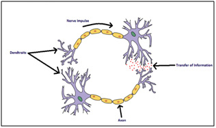Figure 1: Biological Neural Network

Every biological neuron connected to the neighboring neurons and communicate to each other. The axons in the network carry the input-output signals. They receive the inputs from the environment which create the impulse in form of electrochemical signals which travel quickly in the network.A neuron may store the information or it may forward it to the network. They transfer the information to the neighbors through their dendrites.

Artificial neural networks work similarly to the working of biological neural networks. An ANN is an interconnection of artificial neurons. Every neuron in the layer is connected to all the neurons of previous and next layers. There is a weight given as the labels at each interconnection between neurons.Each neuron receives input which is the output of neurons of the previous layer. They process this input and generate an output which is then forwarded to the neurons of next layer. There is an activation function used by each neuron of the network which collects the inputs, sums the inputs and generate the output (Hopfield, 1988). There are various types of activation functions which are chosen on the basis of required output.

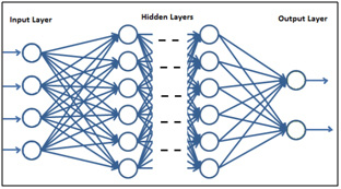
A simple artificial neural network is composed of three layers. The input layer, the hidden layer and the output layer. The inputs in the form of input vector are applied to the input layer. The number of neural nodes in the input layer depends on the number of attributes in the input. The output of each neuron at input layer is forwarded to every neuron of hidden layer where they are received as inputs. The hidden layer is also referred as the processing layer. Because this is the main layer where the processing is performed on inputs. The number of nodes at hidden layer are decided randomly first and it may be adjusted during training. The outputs of each neural node at hidden layer is then forwarded to output layer where they are received as inputs. The output layer then generates the output which is collected as final output of the network. The number of nodes at output layer depends on the type of output(Abraham, 2005). In classification problems, the number of nodes are same as the number of classes the inputs are to be assigned. In regression problems, there may be only output node to produce an output value.

On the basis of layers, there are two types of feed-forward artificial neural networks. The first type is the single layer feed-forward ANN and the second type is the multilayer feed forward neural network. In a single layer, there is no any hidden layer in the network. It is the simplest kind of neural network. The network is composed of the input layer and the output layer only. The inputs applied to the input layers are directly forwarded to the output layer for generating the outputs.

Feed-Forward Artificial
Neural Network

There are various types of artificial neural networks each has a specific property and can be applied in a different problem domain. Feed-forward structure of artificial neural networks have been used very popularly in many applications. A feed-forward network is one where the signals travel in one direction only that is the forward direction, means from the input layer to the output layer (Bebis et al, 1994). There are feed-backward or feedback neural networks which we will discuss later in this chapter. Every neural network works on some learning algorithm.

There are various types of learning algorithms which are selected depending on the problem to which the network is being used. The training of the networks is done by implementing the learning algorithm. Backpropagation learning algorithm is very popular and applied in many applications to train the neural network. It adjusts the weight of interconnections using error in output at a layer. This error is propagated in the backward direction to the previous layers. That is why it is called backpropagation algorithm (Buscema, 1998). There are many other algorithms for each supervised and unsupervised training of the network. The architecture of a feed-forward neural network is represented in figure 2 given below.

Figure 2:  Feed-Forward Artificial Neural Network

In above figure, the architecture of a feed-forward neural network is represented. This network is a composition of artificial neurons where every neuron is connected to the neurons of its previous and next layers. During training of the network, the inputs in form of a vector are applied to the vector of neural nodes at input layer. In many learning algorithms, a bias input is also applied to the main input. This bias value is fixed during the training. The first input pattern is applied and it is transferred to the hidden layer. The activation function used at neurons generate the output which is collected at the output layer. In classification problems, the step functions are generally used and in regression problems, the logistic problems are used. The training of the network is performed on the dataset in many epochs. Some algorithms use gradient descent to stop the training process after reaching to certain error.

Let the inputs I₁, I₂… , I_n are applied to the input layer of the network, then the net input received at a single neuron ofhidden layer is:

Where w is the weight on interconnection and b is the bias value, and hence the net input received at the hidden layer, if there are m neurons, is represented in the form of a vector as:

Let the inputs are represented in the form of the vector as I = (I₁, I₂… , I_n) and W is the matrix of weights associated with the interconnections between the input layer and the hidden layer then Y_in will be defined as the cross product of the input vector and the weight matrix, i.e.,

If f is the activation function used at this neuron, then the output of the neuron is obtained as:

Similarly, the output generated by all the neurons of the hidden layer can be represented in the form of a vector as:

Now, this output Y_out is supplied as input to each neuron of the output layer. Let V is the matrix of weights associated with the interconnections between the hidden layer and the output layer then the input received at output layer will be the cross product of Y_outand V. Let Z_in is the net input received at output layer, then it can be represented as:

Let is the output generated by each of the i^thneuron at output layer and there are p number of nodes are there at this layer, then the net output collected at output layer can be represented as the vector of outputs generated by each neuron. It can be given as:

Activation Functions

Every neuron in the neural network generates the output which is referred as the activation of the neuron. Initially, when the neurons are not generating any output are said to be not activated. When the applied input values reach toa certain threshold, the neurons start firing the output which is called that the neuron is activated. For this activation, a function is used which maps the net input received to the neuron with the output. This function is called the activation function. There are various types of activation functions used at neurons depending on the problem to which the neural network is being applied (Roy, Chakraborty, 2013). The popularly used activation functions are the step function and the sigmoid function. Here we will present a brief description of these functions.

Step Function

There are two types of step functions, the binary step function,and the bipolar step function. The binary step function produces 0 as the output if the net input is less than the certain threshold value è otherwise, it produces 1 as the output.It can be represented mathematically as given in equation 10 and graphically as given in figure 3.

Figure 3: Binary Step Function

The bipolar step function is used when the neural network is to be applied to bipolar data instead of binary data. This function gives -1 and + 1 as the output in place of 0 and 1 depending on the threshold. This function can be represented mathematically as given in equation 11 and graphically as given in figure 4.

Figure 4: Bipolar Step Function

Sigmoid Function

Since the step functions are not continuous, so they are not differentiable. There are some machine learning algorithms which require the continuous and differentiable activation functions and hence the step functions cannot be used in those problems. The sigmoid functions can be approximated with maintaining their property of differentiability. There are two types of sigmoid functions used in this type of problem domain, the binary sigmoid function,and the bipolar sigmoid function. They both have the continuous outputs.

The binary sigmoid function is also called the logistic sigmoid function. It can be represented mathematically as given in equation 12 and graphically as given in figure 5.

Figure 5: Binary Sigmoid Function

where á is called the steepness parameter.

The binary sigmoid function has the limitation that it cannot be applied to bipolar data. In this case, the bipolar sigmoid function is used for continuous output. It can be represented mathematically as given in equation 13 and graphically as given in figure 6.

Figure 6: Bipolar Sigmoid Function

Learning By Anns

An artificial neural network has three important characteristics, the architecture, the activation function and the learning. The weights associated with the interconnection between neurons of the network are initialized randomly before training of the network. These weights are adjusted by following the learning algorithm and when finalized, the network is said to be a stable of the fitted network. A network fitted after training can be applied to a problem (Haykin, 1998). During training, the weights of the neural network are updated at each iteration of the training until some stopping condition is satisfied. Let w(k) is the weight at k^th iteration of the training then the new weight at (k+1)^st is obtained as given in the equation 14.

where the ∆w(k) is the change in weight w at k^th iteration. Different learning methods give a different method to obtain the ∆w(k).

There are various learning methods used by neural networks which are categorized mainly into two categories, the supervised learning and the unsupervised learning (Jain et al, 1996).

Supervised Learning

The supervised learning methods work with the labeled data. Labeled data means the data where there are input and output labels given in the data. The training data for a neural network is referred as the training pattern. Each training pattern consists of the input patterns and corresponding output patterns in case of supervised learning. The learning algorithms devise a function mapping between the input and output patterns of the data. Once the network is trained by following the learning algorithm, it can generate output for an unknown input pattern (Reed et al, 1999). Here we will present a very brief description of the supervised learning algorithms popularly used in the training of neural networks.

Hebb Rule

It is one of the earliest learning algorithms used by the artificial neural networks. According the Hebb rule or Hebbian learning, the change in weight w_i can be obtained as:

where I_i is the corresponding input value and the t is the target value. The Hebb rule has the limitation that it cannot learn if the target is 0. This is because the change in weight ∆w_i will become 0 when we put t=0. So it is applied when the input and output both are in bipolar form (Kempter et al, 1999).

Perceptron Learning Rule

According to the perceptron learning, if the output of the neuron is not equal to the target output, then only the weights associated with the interconnections should be adjusted otherwise they should not be altered (Nget al, 1997). According to this rule, the change in weight w_i is obtained as:

where ç is a constant and known as the learning rate.

Delta Rule

The Delta rule is also known as the Least Mean Square (LMS) or Widrow-Hoff rule. It is a widely used learning method used in the training of neural networks. It produces the output in binary form by reducing the mean squared error between the activation and the target value (Auer et al, 2018). According to the Delta rule, the change in weight ∆w_i is obtained as:

where the symbols used have their usual meaning.

The Backpropagation Algorithm

The backpropagation is the most popular learning algorithm used for training the artificial neural network in case of supervised learning. In this algorithms, the neural net repeatedly adjusts the interconnection weights on the basis of error and deviation from the target output in response to the training patterns. The error in this method is calculated at the output layer of the network and propagated back through the network layers (Adeli et al, 1994). We will discuss this method in detail in chapter 6 while discussing the training of Hybrid Deep Neural Network.

Unsupervised Learning

When the training data available for training the neural network does not has the input-output labels, the learning performed on this data is called the unsupervised learning. In this case, the algorithms learns to derive structure from the data. There are many machine learning problems like clustering and anomaly detection use unsupervised learning (Hastie et al, 2008). In clustering problems, during training of the neural network, the input vectors which are to be applied to the network are combined to form clusters. When the network is trained or stable, on applying a new input vector, the neural network gives the output response indicating the cluster to which the input vector belongs.The popular unsupervised learning algorithm used for clustering using neural network is Winner-Takes-All method. It is a competitive learning rule which chooses the neuron with the greatest total input as a winner (Kaski et al, 1994).

Deep Learning Models

There are various deep learning models developed by the researchers and they are applied in a different problem domain. In all the models, the common characteristic is the multiple layers of learning. Here in this section, we will present a short survey of popularly used deep learning models.

Deep Neural Network

Deep neural network is a variant of multilayer feed-forward artificial neural network. It has more than one hidden layers between the input layer and the output layer (Bengio, 2009). The number of neurons are similar in each of the hidden layer. Initially, the number of neurons are fixed randomly and it is adjusted manually during training of the network. Larger the number of nodes at hidden layer may result in an increase in the complexity and hence the decrease in the training performance. So, the selection of number of nodes at this layer is carefully considered. This architecture devises a compositional model in which the object is referred as the layered composition of primitives. It has the capability to model complex non-linear relationships in the training data. The benefit of using extra hidden layers in the network enables the composition of features from lower layers. These features potentially model complex data with fewer units (Ngiam et al, 2011).

There are two issues also associated with the deep neural networks. First, the issue of overfitting which is common in many neural network models and second, the issue of computation time. The problem of overfitting has more chances to arise in deep neural network due to the use of extra layers. Due to this issue, it models the rare dependencies in the training data. The network gives better result on training data and degraded in accuracy on validation data. To avoid the issue of overfitting in deep neural networks, regularization methods like weight decay or sparsity can be used during training which excludes the modeling of rare dependencies. With the increase in smaller training sets can also overcome the problem of overfitting. The computation time of the learning model depends on many parameters like such as the layer size, the learning rate, and the initially chosen weights (Szegedy et al 2013). The number of nodes in the hidden layers increase the complexity of the system and it requires more computational time. It should be carefully considered while selecting all these
parameters.

A typical architecture of the deep neural network is represented in figure 7.

Figure 7: Deep Neural Network

All the processing in the deep neural network is very much similar to the multilayer feed-forward artificial neural networks. For training of the network, the backpropagation learning method is used widely to find the matching between the actual output and the desired output. The change in weight in this process is calculated as:

where ç is the learning rate, C is the cost function and î is the stochastic term. w_ij is the weight associated with the interconnection between i^th node of one layer and j^th node of next layer.

The deep neural networks have a wide range of applications. They are applied in automatic speech recognition, image recognition, visual art processing, and natural language processing, drug discovery, customer relationship management, mobile advertising and many more fields.

Convolutional Neural Network

The convolutional neural network is a variant of a multilayer perceptron. They are inspired by the biological process of visualization. This model is a composition of neurons, learnable weights, and bias values. It consists of an input layer, an output layer and multiple hidden layers between the input layer and the output layer.The hidden layers of the network are the composition of the convolution layers, pooling layers, fully connected layers and the normalization layers. They are designed in such a manner that they require a minimal amount of preprocessing (Aghdam, 2017, Krizhevsky et al 2012). The architecture of a convolutional neural network is represented in figure 8 given below.

Figure 8: Convolutional Neural Network

The architecture of convolutional neural network comprises neurons in three dimensions, the depth, the height and the width which are presented in one of the layers. The 3D input volume is transformed to 3D output volume of neuron activations by every layer of the network. A typical architecture of convolutional neural networks consist of the following:-

(i). Convolutional Layer

The convolutional layer of the network is termed as the core building block which comprises a set of learnable filters. It is said that these filters are convolved around the layer. It applies a convolution operation to the input which is to be passed to the next layer as a result of this operation. The network learns from the filters as they are activated after detecting certain specific type of features at certain spatial input position.

(ii). Pooling Layer

Pooling layer helps the convolutional neural network in avoiding the issue of overfitting which is a common issue in artificial neural networks. Pooling, which is a form of non-linear down-sampling, combines the outputs of neurons of one layer into a single neuron of next layer. The max-pooling partitions the input data into a set of non-overlapping slices and produces the maximum output for each set.

(iii). Local Connectivity

In convolutional neural networks, neurons of one layer are connected only to the neighboring neurons of adjacent layers. When dealing with the input of high volume, this features avoids the problem of connectivity and hence reduces the complexity of the network.

(iv). Parameter Sharing

There is a feature of parameter sharing in convolutional neural networks which helps in controlling the free parameters. Weight vectors and bias values are shared among the neurons of the network which helps in less parameter optimization and faster convergence during training.

In the field of natural language processing, convolutional neural networks are applied to text analytics and sentence classification problems (Kalchbrenner et al, 2014). Itis also used in the time-series analysis which is helpful in predicting stock prices, heights of ocean tides and weather (LeCun et al, 1998). The architecture of convolutional neural network has been used in predicting the DNA sequence binding (Zeng et al, 2016). These architectures are also used in drug discovery by predicting the interactions between biological proteins and molecules (Strigl et al, 2010).

However convolutional neural networks have been applied very usefully in many fields and they have given better results, some limitations are also associated with this model. It requires a large data set and hence needs a long training time. There is the issue of performance and scalability also associated as this architecture is GPU based (Hinton, 2009).

Deep Belief Networks

A deep belief network is a variant of the deep neural network. It is a graphical model which is composed of multiple layers of hidden units. The hidden units are called the latent variables. There is an interconnection between layers of the network but there is no connectivity among units of the network. This graphical model learns to extract the deep hierarchical representation of the training data (Hinton et al, 2006). The graphical model has both directed and undirected edges. The training of the network is performed in two successive steps, the unsupervised training and then thesupervised training. During the unsupervised training, the network learns to probabilistically reconstruct its inputs when trained on a set of example. As a result of this training step, the layers act as feature detectors. After this step, the supervised training is performed on the network to perform the task of classification (Salakhutdinov et al, 2007).

The deep belief network can be described by separating its architecture in two parts, the belief network,and the Restricted Boltzmann Machine. The belief network is a directed acyclic graphical model comprises the stochastic variables. These variables have states either 0 or 1 where the probability of becoming 1 is obtained by a bias and weighted inputs from other units. The belief network solves two types of problems, the inference problem,and the learning problem. The inference problem infers the state of the unobserved variables and the learning problem adjusts the interconnection between learning variables. This helps the network in generating the observed data. The Restricted Boltzmann Machines are the generative models of the artificial neural network which learns from the probability distribution of a set of inputs (Larochelle et al, 2008).

A typical architecture of deep belief network is represented in figure 9.

Figure 9: Deep Belief Network

The deep belief network is composed of Restricted Boltzmann Machine (RBM) and a feedforward multilayer perceptron. The RBM is used at pre-training phase and the multilayer perceptron is used at the fine tune phase. The hidden units of the network are the neurons which cannot be observed directly but they can be inferred from the other observable variables. In deep belief networks, the distribution between observed input vector X and n^th hidden layer h_nis modeled as:

where, X= h₀, P (h_i-1,h_i) is a conditional distribution of visible units and P (h_n-1,h_n) is the joint distribution for visible units. During the first step of the training, the network learns a layer of features from the visible units. Then, in the next step, it treats the activation of previously trained feature as visible unit and learns features in a second hidden layer. After following successive steps in such manner, the whole network is said to be trained when the learning for the final hidden layer is achieved.

Deep Belief Networks have been used in financial business predictions in order to empower the financial industries. These networks have also been used in time series prediction which then leads to financial market, signal processing,and weather information prediction. Draught has also been predicted by this model. It is also used in predicting the quality of sound vehicle interior noise (Medsker et al, 2001).

However, Deep Belief Networks have a wide range of application, some limitations are also associated with this model. Since deep belief networks are formed with Boltzmann Machines, they have the limitation that when the size of the machine is increased, the training time of the model exponentially increased.

Recurrent Neural Networks

Recurrent neural network belongs to the class of artificial neural network. In these networks, there is a directed cyclic connection between its internal nodes along a sequence. It exhibits the dynamic temporal behavior of a time sequence. These networks use internal memory states to process in the input sequences (Li et al 2015). In conventional artificial neural networks, input values in an input vector are independent of eachother and hence processed independently. But there are many tasks where the output is dependent on previous calculation in a sequential process. The recurrent neural networks are applied to such type of tasks where there is sequential process on inputs. This network is called recurrent because it performs the same task for every element in the sequence. The memory used by the network stores the information about previous calculations. Practically, these networks recall calculations of few previous steps only (Schuster et al, 1997).

The working of the recurrent neural network can be explained by the architecture represented in figure 10 given below.

Figure 10: Recurrent Neural Network

The above representation shows a recurrent neural network being unfolded into a full network to process a sequence of inputs. Here, one layer works for each input value in the sequence. If folded or combined all the layers together as a single hidden layer, the weights and bias remain same because of only one hidden layer is used in the network. Let x_t is an input to the network at timestamp t and s_tis the hidden state or memory at timestamp t. This s_t is calculated on the basis of hidden state at previous timestamp and the input at current timestamp as

where f is a nonlinear function which may be tanh or ReLU. s_t-1 is initialized to zero at first timestamp. o_t is the output at t timestamp which is calculated as

in the above equation 4.21, f is a logistic function which may be softmax or a normalized exponential
function.

Unlike the other deep neural networks where different parameters like weights and bias are used at different hidden layers, in the recurrent neural network these parameters are shared across all the timestamps. This helps in reducing the number of parameters during learning. In some applications, there is input required at each timestamp and there is an output produced at each timestamp. But it is not necessary in every application of recurrent neural network. This because of the use of hidden state which captures information about some sequences.

There are multiple extensions of the recurrent neural network. They are discussed briefly as given below.

• Bidirectional Recurrent Neural Networks

This network is based on the concept that the output at t timestamp is not only dependent on the previous elements in the sequence but it also depends on the future elements. It architecture is such as two recurrent neural networks are stacked on top of eachother. Its output is calculated based on the hidden state of both networks (Irsoy et al, 2014).

• Deep Bidirectional Recurrent Neural Networks

These networks are similar to the bidirectional recurrent neural networks with an addition that they have multiple layers per timestamp. It gives the benefit of higher learning capacity but it needs a large size of training data (Hochreiter et al, 1997).

• Long Short-Term Memory (LSTM) Networks

This variant of the recurrent neural network is applied to avoid the vanishing gradient problem in backpropagation learning. In these networks, the memory units are called as cells which are very efficient to capture long-term dependencies. It takes the previous state s_t-1and current input x_tas input to the cells and these cells decide internally that which information will be stored and which information will be erased (Saad et al, 1998).

Recurrent Neural Networks have a large number of applications in predictive analytics. It has been widely used in stock market predictions for a long period of time (Connor et al 1994). Its application in time series prediction has given the generalization of performance than other models (Hu et al, 2007). These networks, after combining dynamic weights, have been used to predict the reliability of the software (Barbouniset al 2006). With the addition of spatial correlation features, the recurrent neural network is used to predict the speed of wind (Levin, 1990).

Apart from the above important applications, RNNs have some limitations. There is a slow training time of these networks. In RNNs, number of hidden neurons must be fixed before training. While processing a vocabulary, size of context must be small (Sundermeyer et al, 2013).

Conclusion And Future Scope

In this paper, we have discussed the various techniques used in deep learning applications. All these models have an outstanding record in the area of machine learning. There is a scope to create new features in these models so that they can be applied in many domains with better performance. The new techniques may be integrated to exploit the opportunities of the model in prediction. Parameter tuning can also help to improve the performance of these models. Parameter tuning can also help to improve the performance of these models. So it can be said that there is a very wide opportunity and open scope for this model.

References

Abraham A (2005) Artificial Neural Networks. Handbook of Measuring System Design, Willey Online Library.

Adeli H and Hung S-L (1994) Machine learning: neural networks, genetic algorithms, and fuzzy systems. John Willey & Sons.

Aghdam H H and Heravi E J (2017) Guide to convolutional neural networks: a practical approach to traffic sign detection and classification. Springer Publication.

Auer P, Burgsteiner H and Maass W (2018) A learning rule for very simple universal approximators consisting of a single layer of perceptrons in Neural Networks Vol. 21 Issue 5: Pages 786-795.

Barbounis T G, Theochairs J B, Alexiadis M C and Dokopoulos P S (2006) Long-term wind speed and power forecasting using local recurrent neural network models in IEEE Transactions on Energy Conversion Vol. 21 Issue 1: Pages 273-284.

Bebis G and Georgiopoulos M (1994) Feed-forward neural networks in IEEE Potentials Vol. 13 Issue 4: Pages 27-31.

Bengio Y (2009) Learning Deep Architectures for AI in Foundations and Trends in Machine Learning Vol. 2 Issue 1: Pages 1-127.

Buscema M (1998) Back Propagation Neural Networks in Substance Use & Misuse Vol. 33 Issue 2: Pages 233-270.

Chen X-W and Lin X (2014) Big Data Deep Learning: Challenges and Perspectives in IEEE Access Vol. 2.

Connor J T, Martin R D and Atlas L E (1994) Recurrent neural networks and robust time series prediction in IEEE Transactions on Neural Networks Vol. 5, Issue 2: Pages 240-254.

Deng L and Yu D (2014) Deep Learning: Methods and Applications in Fundamentals and Trends in Signal Processing, Vol. 7 Issue 3: Pages 197-387.

Garven M V and Bohte S (Accessed 2018) Artificial Neural Networks as Models of Neural Information Processing. Frontiers Research Topics, Online.

Goodfellow I, Bengio Y andCourville A (2016) Deep Learning. MIT Press, Online.

Hastie T, Tibshirani R and Friedman J (2008) Unsupervised Learning. The Elements of Statistical Learning Springer Series in Statistics: Page 485-585.

Haykin S (1998) Neural Networks: A Comprehensive Foundation. Prentice-Hall, 2^nd Edition.

Hinton G (2009) Deep Belief Networks in Scholarpedia, Vol. 4, Issue 5.

Hochreiter S and Schmidhuber J (1997) Long Short-Term Memory in Neural Computation Vol. 9 Issue 8: Pages- 1735-1780.

Hinton G E, Osindero S and Teh Y W (2006) A Fast Learning Algorithm for Deep Belief Nets in Neural Computation Vol. 18 Issue 7: Pages 1527-1554.

Hoff R D (Accessed 2018) Deep Learning: A Breakthrough Technology. MIT Technology Review, Online.

Hopfield J J (1988) Artificial neural networks in IEEE Circuits and Device Magazine Vol. 4 Issue 5: Pages 3-10.

Hu Q P, Xie M, Ng S H and Levitin G (2007) Robust recurrent neural network modelling for software fault detection and correction prediction in Reliability Engineering and System Safety Vol. 92 Issue 3: Pages 332-340.

Irsoy O and Cardie C (2014) Opinion Mining with Deep Recurrent Neural Networks in Proceedings of the 2014 Conference on Empirical Methods in Natural Language Processing (EMNLP): Pages 720–728.

Jain A K, Mao J and Mohiuddin K K (1996) Artificial neural networks: a tutorial in Computer Vol. 29 Issue 3: Pages 31-44.

Kalchbrenner N, Grefenstette E andBlunsom P (2014) A Convolutional Neural Network for Modelling Sentences in Proceedings of the 52^nd Annual Meeting of the Association of Computational Linguistics, Baltimore, Maryland: Pages 655-665.

Kaski S and Kohonen T (1994) Winner-take-all networks for physiological models of competitive learning in Neural Networks Vol. 7 Issue 6: Pages 973-984.

Kempter R, Gerstner W and Hemmen J L (1999) Hebbian learning and spiking neurons in Physical Review E Vol. 59 Issue 4: Pages 4498-4514.

Krizhevsky A, Sutskever I and Hinton G E (2012) ImageNet Classification with Deep Convolutional Neural Networks in Proceedings of Advances in Neural Information Processing Systems 25.

Larochelle H and Bengio Y (2008) Classification using discriminative restricted Boltzmann machines in Proceeding of 25^th International Conference on Machine Learning, Finland: Pages 536-543.

LeCun Y and Bengio Y (1998) Convolutional networks for images, speech, and time series in The handbook of brain theory and networks: Pages 255-258.

Levin E (1990) A recurrent neural network: Limitations and training in Neural Networks Vol. 3 Issue 6: Pages 641-650.

Li X and Wu X (2015) Constructing long short-term memory based deep recurrent neural networks for large vocabulary speech recognition in Proceedings of the IEEE International Conference on Acoustics, Speech and Signal Processing, QLD, Australia.

Medsker L R and Jain L C (2001) Recurrent Neural Networks: Design and Applications. CRC Press LLC.

Najafabadi M M, Villanustre F, Khoshgoftar T M, Seliya N, Wald R and E Muharemagic (2015) Deep learning applications and challenges in big data analytics in Journal of Big Data Vol. 2 Issue 1: Pages 1-21.

Ng H T, Goh W B and Low K L (1997) Feature selection, perceptron learning, and a usability case study for text categorization in Proceedings of the 20th annual international ACM SIGIR conference on Research and development in information retrieval, Philadelphia, Pennsylvania, USA: Pages 67-
73.

Ngiam J, Khosla A, Kim M, Nam J, Lee H and Ng A (2011) Multimodal Deep Learning in Proceedings of 28^th International Conference on Machine Learning, WA, USA.

Nisbet R, Miner G and Yale K (2018) Chapter-19, Deep Learning. Handbook of Statistical Analysis and Data Mining Applications, 2^nd Edition, Academic Press.

Reed R and Marks R J (1999) Neural Smithing: Supervised Learning in Feedforward Artificial Neural Networks. A Bradford Book, MIT Press.

Roy S and Chakraborty U (2013) Introduction to Soft Computing: Neuro-Fuzzy and Genetic Algorithms. Pearson Education India, 1^st Edition.

Saad E W, Prokhorov D V and Wunsch D C (1998) Comparative study of stock trend prediction using time delay, recurrent and probabilistic neural networks in IEEE Transactions on Neural Networks Vol. 9 Issue 6: Pages 1456-1470.

Salakhutdinov R, Mnih A and Hinton G (2007) Restricted Boltzmann machines for collaborative filtering in Proceeding of 24^th International Conference on Machine Learning, Oregon, USA: Pages 791-798.

Schuster M and Paliwal K K (1997) Bidirectional recurrent neural networks in IEEE Transactions on Signal Processing, Vol. 45 Issue 11: Pages 2673-2681.

Strigl D, Kofler K and Podlipnig S (2010) Performance and Scalability of GPU-based Convolutional Neural Networks in Proceedings 18^thEuromicro International Conference on Parallel, Distributed and Network-Based Processing, Pisa, Italy.

Sundermeyer M, Oparin I, Gauvain J-L, Freiberg B, Schluter R and Ney H (2013) Comparison of feedforward and recurrent neural network language models in Proceedings of the IEEE International Conference on Acoustics, Speech and Signal Processing, BC, Canada.

Szegedy C, Toshev A and Erhan D (2013) Deep Neural Networks for Object Detection in Proceedings of the Advances in Neural Information Processing Systems 26.

Yegnarayana B. Artificial Neural Networks. Prentice-Hall of India, Latest Edition.

Zeng H, Edwards M D, Liu G and Gifford D K (2016) Convolutional neural network architectures for predicting DNA-protein binding in Bioinformatics Vol. 32 Issue 12: Pages 121-127.