Department of Electrical Engineering, Kerman Branch, Islamic Azad University, Kerman, Iran
Corresponding author Email: h.zayandehroodi@yahoo.com
Article Publishing History
Received: 19/03/2017
Accepted After Revision: 22/06/2017
The present work was formulated in order to obtain proper amount of load needed in Bafgh for 2017. The study was performed in five sectors, i.e. industry, household, business, public, and agriculture. After obtaining the results relative to load prediction for Bafgh, optimization of a compound generator system (wind and solar) independent of the network was considered for this city. The results showed that Bafgh needs 368,976 (MW) per hour in 2017. The results indicate the necessity of governmental support in private sector in establishment of such systems. The results obtained from optimization indicated that use of renewable energies increase if subsidies are completely removed so that generator diesel production will decrease as fuel price increases. The recommended system in the present work can be the best solution for Bafgh in 2017.
Wind Turbine – Load Prediction – Solar Array-Diesel Gen
Goughari R. S, Zayandehroodi H, Eslami M. Environmental Oriented Optimal Selection of Renewable and Green Energy Sources Using Intelligent Methods: A Case Study of Bafgh – Iran. Biosc.Biotech.Res.Comm. 2017;10(2).
Goughari R. S, Zayandehroodi H, Eslami M. Environmental Oriented Optimal Selection of Renewable and Green Energy Sources Using Intelligent Methods: A Case Study of Bafgh – Iran. Biosc.Biotech.Res.Comm. 2017;10(2). Available from: https://bit.ly/2YccH12
Introduction
In The study forecast load is performed once for the city Bafgh in 2017. The forecast five trade tariffs, domestic, industrial, agricultural and made public. This prediction using neural network software SPSS Tool is available in this software. Data used in this study include daily load for the past five years. All economic and social activities of society are dependent on electric industry. With regard to the fact that electric energy cannot be stored in a large scale and that various projects of electric industry demand long-term planning, a suitable estimation for different parts of power systems is very important. Optimal design of a power system is possible when economic, technical, and environmental issues are accurately considered. Therefore, the most important part of a power system is prediction of load (Ghanbari, et al. 2009).
Planning for energy supply for next generations is one of the most crucial concerns of governments. The planning calls for suitable estimation of power systems’ demands in future. The planning is performed in three parts, i.e. load prediction, production planning, and transmission planning. The most important part of planning in a power system is load prediction. Due to its high capability in learning and relationship between inputs and outputs, neural network is one of the most efficient methods.
Neural networks are inspired from information processing from biologic neural system and processes information as brain does. Key element of the idea is the novel structure of information processing system; the system is comprised of several processing elements which coordinately work for problem solving (Passino, 2002).Like humans, Artificial Neural Networks (ANNs) learn by examples. An ANN is adjusted for performing a known task such as recognition of patterns and classification of data during a learning process. In biologic systems, learning is accompanied by adjustments in synaptic connections between nerves (Lakshminarasimman and Subramanian 2008).
The present work was formulated in order to obtain proper amount of load needed in Bafgh for 2017. The study was performed in five sectors, i.e. industry, household, business, public, and agriculture. The estimation was executed in order to prevent from occurrence of troublesome conditions in network such as overload in lines, network failure, etc. it is possible to increase confidence level of network in this city so that electrical sector’s authorities can have suitable programs in different parts of electrical industry in Bafgh on the basis of the results of the present work. After obtaining the results relative to load prediction for Bafgh, optimization of a compound generator system (wind and solar) independent of the network was considered for this city.
A technique for the optimal planning and design of hybrid renewable energy systems for microgrid applications is presented in (Jung, et al. 2016); a novel approach is used to determine the optimal size and type of distributed energy resources (DERs) and their operating schedules for a sample utility distribution system. The 4 main aspects for energy efficiency in a building consist of first the nearly zero energy passive building design before actual construction, secondly the employment of low energy building materials during its construction, thirdly use of energy efficient equipment for low operational energy requirement while lastly integration of renewable energy technologies for various applications. These aspects along with their economics and environmental impacts are discussed by Chel, et al. (2017).
Recently, Hong, et al. (2017) have investigated the optimal sizing of renewable energy generation resources in a community microgrid; the cost of renewables and community welfare are optimized while the comfort zone of indoor temperature in all houses is maintained using air conditioning systems. Similarly, Tezer, et al. (2017) have also with the aim of investigating optimization techniques, developed from past to present to solve the problems of stand-alone hybrid renewable energy systems and especially have tried to determine the efficacy of multi-objective optimization approaches.
Materials and Methods
Neural network estimations in SPSS
SPSS Software (Statistical Package for the Social Sciences) can be adopted to run prediction through neural network imbedded inside the software. Here, weight coefficient and role of each independent variable are determined in prediction of dependent variable by using toolbar of neural network (Chen, 2000).
| Table 1: The results of neural network analysis | |
| Characteristics Amount | |
| Number of middle layers 1 | |
| Number of middle units 2 | |
| Trainig | Data volume 70% |
| Sum of squared errors 31.131 | |
| Relative error 0.0988 | |
| Test Data volume 30% | |
| Sum of squared errors 21.484 | |
| Relative error 0.996 | |
Neural network architecture
Although neural networks do not need preconditions and model structures very much, it is still effective to grasp a whole definition of network architecture. MLP and RBF are functions of predictors minimizing prediction error of target variables (Chen, 2000). Figure 1 depicts an example of a neural network used to choose optimal plants of distributed production.
 |
Figure 1: Neural network structure for choosing optimal plants of distributed production |
The above architecture is known as Feed Forward Architecture because intra-network relationships are directed forward from input layer toward output layer without any return. In this figure, input layer consists of predictors; input layer consists of knots or invisible units. Value of each hidden unit depends on predictors. Accurate architecture of function is related to two dependent factors, i.e. network type and controllable characteristics by user; output layer consists of reactions.
MLP Network enables having two hidden layer; in this case, each unit in the second hidden layer is a function of existing layers in the first hidden layer and each response is a function of units of second hidden layer’s units. MLP method provides a predicting model for one or some dependent variable(s) (target) according to values of predictor variables (Ghanbari, et al. 2009).
Dependent Variables
The following scales can be considered here: (a) Nominal scale: Letters are used to measure variable; (b) Ordinal scale: There is an order among variable levels, e.g. 5-choice scale (very low, low, average, high, and very high) ; (c) Interval scale: Zero is conventional and the interval between two consecutive units is a constant value, e.g. Fahrenheit and Centigrade; (d) Ratio scale: It is similar to interval scale, the only difference is that Ratio scale’s zero is real, e.g. centimeter and inch. In the above-mentioned steps, it is postulated that a proper level of measurement is given to all dependent variables. Nevertheless, measurement levels for a given variable can be changed by right-clicking on the variable in the list and choosing a measurement level from the list. A pointer beside each variable in variable list determines measurement level and type of data (Chen, 2000).
Predictor Variables
Predictors may be determined categorically or relatively. Categorical variable coding of the process temporarily recodes categorical predictor and dependent variables by using one of “c” codes until the end of the steps. If there are c categories of a given variable, they are saved as c vectors. This model of coding increases synaptic weights and slows down training. However, the more intensive the coding methods are, the weaker conformity with neural network will be achieved.
Creating an MLP neural network in SPSS Software
Variables
Neural networks and then Multilayer perceptron are chosen from Analyze menu in SPSS. Dependent variables and covariates are chosen.
On the Variable bar, rescaling of covariates is changed. The choices are as follows:
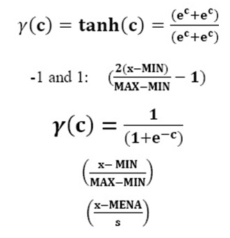
9 Standardized: Subtract the mean and divide it by standard deviation
(1)
9 Normalized: Subtract the minimum value and divide it by range:
(2)
9 Adjusted normalized: A sample is set from normalized values between
(3)
9 None : no rescaling of covariates.
Partitions
The Partitions part is used to separate Training and Test data. It is recommended to use 70% of data for network training and 30% of them for network test to select optimal plants of distributed production.
Architecture
Network architecture is decided in this part. This menu automatically assigns the best architecture.
9 Activation function
The Activation function relates weighed sum of units in one layer to unit values of next layer:
Hyperbolic tangent : The function receives real values and turns them in (-1,1) interval. The function is as follows:
(1)
Sigmoid: The function receives values and turns them in (0,1) interval. The function is as follows:
(2)
The Output layer consists of dependent variable (target variable). Activator function makes a relationship between weighed sum of units in one layer and values of next units.
- Identity : The function receives real values and returns them without any change.
- Soft max: This function receives real values and turns them to a vector.
- Hyperbolic tangent: this function receives real values and turns them in (-1,1) interval.
- Sigmoid: This function receives real values and turns them in (0,1) interval.
The Rescaling of scale dependent variables
- Standardized: Mean is subtracted and the result is divided by standard deviation.
- Normalized: The minimum value is subtracted and the result it is divided by range; the normalized values are in (0,1) interval.
- Adjusted normalized: The minimum value is subtracted and the result is divided by range. The adjusted normalized value is in (-1,1) interval.
- None: No rescaling of scale dependent variables.
Training
With regard to type of training, one of the following types is selected (Elizabeth, et al. 1995, Mandal, et al. 2006).Table 1: The results of neural network analysis
Batch
The Batch brings synaptic weights up-to-date for training only after determination of all saved data. In other words, training a batch of data related to all saved values in databank is preferred because it minimizes total error. Batch training needs to be updated several times to reach one of criteria of weights cease; therefore, the databank should be checked several times. This method is more suitable for smaller groups of data.
Online
The Online brings synaptic weights up-to-date after each saved training data. In other words, online training uses the information related to a save in a time. Online training gets a save frequently and updates weights in order to reach a criterion of cease. If all saves are used once and no cease criterion is met, processing continues with recovering information saves. Online training has a better performance than batch method in bigger information sets with related predictors. If there are several saves and variables and their values are related to each other, online training archives acceptable response in a shorter period of time.
Mini-Batch
Test data are classified into almost same groups and then updating is performed on synaptic weights after passing a group. That is, the Mini-Batch method makes use of the information from a saved group; then, the process recovers group data if necessary. Mini-Batch training is in fact an agreement between batch and online training and it is considered the best method for medium-sized information banks. In this method, the program can assign the number of saved data automatically for training and therefore, a value >1 or ≤max. Number of cases is decided to be saved. Maximum number of saved cases can be specified in the option bar (Mandal, et al. 2006).
The data from electric power distribution companies north of the province is taken. Data are divided into two groups of training and test data for classification. For this aim, 70% of data are used for network training and 30% of them are used for test. Multi-Layer Perceptron (MLP) and Radial Basis Function (RBF) are used as neural networks. They compare the prediction results from the model with target values, (Table 1) show the results of neural network analysis. Neural network enables us to adjust MLP and RBF networks and save model results for scoring (Norusis, 2011).
Optimization Algorithm
The Optimization algorithm is a method for estimation of synaptic weights:
Scaled conjugate gradient: Hypotheses of this method enable use of it only for batch training Gradient descent: this method should be used for online and/or mini-batch trainings and it may also be used for batch training (Mandal, et al. 2006).
Training Option
It enables us to adjust optimization algorithm carefully. This part for scaled conjugate gradient consists of the followings:
Initial lambda: Initial lambda in numerical algorithm is assigned between 0< x <0.0000001. Initial sigma: Initial sigma is assigned between 0< x <0.00001 Output Layer
The output layer contains the target variable (dependent) and functions actively between units in a layer the sum of the weighted values of the next relationship.
- 9 Identity: The function of the real values and returns them unchanged.
- 9 Soft max: It function real values and converts them to vector.
- 9 Hyperbolic tangent: this function receives the actual values to the values in the interval (1, -1) turns.
- 9 Sigmoid: This function receives the actual values and the values in the interval (1, 0) converts.
Network Structure
- Description: It shows the information related to neural network consisting of dependent variables, number of input and output units, number of hidden layers and units, and activator functions.
- Diagram: It shows the network like an unchangeable graph.
Synaptic weights: It shows the coefficients estimated for showing the relationship between a layer and the next one even if active information banks are assigned to training data.
- Network performance:
It presents the results used for showing soundness of the model.
- Model summary: It presents a summary of the results on neural network in a complete and separated manner.
- Classification results: It presents a classified table for each dependent variable partially or fully.
- Roc curve: It presents roc dependent curve and a table showing the value under the curve for each dependent variable.
Cumulative gain chart: It shows a cumulative gain chart for each dependent variable.
- Lift chart: It presents a lift chart for each definite dependent variable.
Predicted by observed chart: It present a predicted by observed chart for each dependent variable.
- Residual by predicted chart: It presents residual by predicted chart for each dependent variable.
- Case processing summary: It shows a table consisting of case processing summary. Independent variable importance analysis: It estimates effect of each predictor in determination of neural network and then, presents a table and a chart showing the importance of each predictor (Mandal, et al. 2006).
The Save Menu
- Save predicted value or category for each dependent variable:
It saves predicted values of each dependent variables as well as predicted category.
- Save predicted pseudo-probability or category for each dependent variable:
It saves predicted pseudo- probability for each dependent variable.
- Option:User-missing value: in order for factors to enter analyses, they should have available values. The controls enable us to decide about availability of user-missing values in dependent variables and factors. Maximum training time:
It assigns maximum training time which is >0.
- Maximum Training Epochs:
If maximum training epochs are exceeded, training will stop
- Minimum Relative Change in training error:
If it is smaller than last step, a >0 value is assigned. If test data are only used for estimation of error for online and mini-batch training, the scale will be neglected.
- Minimum Relative Change in training error ratio:
If it is smaller than the given value, the training will stop. After performing the mentioned steps, the results obtained from prediction of neural network are inserted in the main page of the software and other results and characteristics are shown in another file (Arrillaga, 1991).
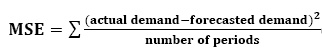
Mean Squared Error (MSE)
- 9 MSE is the average of all of the squared errors.
- 9 it magnifies the errors by each of the error.
the forecast with the smallest MSE best fits the data
The Resources To Be Used In The Software Homer
- Solar resources
- Water resources
- Wind resources
- Biomass resources
- Fossil resources.
In the Homer, attribute is a part of power system which is producer, presenter, converter, or saver of energy. There are ten attributes in the Homer, three of which produces electric power by renewable resources, i.e. wind, solar, and water resources. Three types of generators are networks and boilers which are predisposed to dispatch, that is, system can control them if necessary. Two other types of attributes, i.e. converters and electrolysis, convert electric energy to another form of energy. Two more attributes are batteries and energy saving tanks. The Homer enables users to compare several design choices according to technical and economic principles (Lippman, 2004).
Results and Discussion
Bafgh is a city in and the capital of Bafgh County, Yazd Province, Iran. At the 2006 census, its population was 30,867, in 7,919 families. It is very necessary to make use of clean energies in this city in order to prevent from environmental pollutions and economic considerations. Figures 2 and 3 depict wind speed profile and solar horizontal radiation for Bafgh, respectively. This software is able to analyze and model connected and/or separated systems to mobile electric network with various blends of solar and wind arrays, small water resources, biomass resources, diesel generators, and batteries. The main ability of this software is to simulate long-term behavior of small power systems. In the Homer, equipment price, equipment longevity, fuel price, and geographical and climatic characteristics. Finally, the software selects optimal system according to all predefined conditions with the lowest process
 |
Figure 2: |
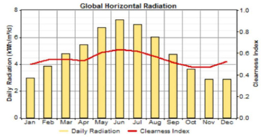 |
Figure 3: Solar horizontal radiation in bafgh |
The forecast five trade tariffs, domestic, industrial, agricultural and made public. According to the above charts. This prediction using neural network software SPSS tool is available in this software. Data used in this study include daily load for the past five years (Mandal, et al. 2006).
Prediction results in different sectors show that effect targeted subsidies were not the same on various sectors. Also, it was found that effect of targeted subsidies in the first year was higher on load profile. However, such factors as appearance of electric agricultural wells have had adverse effect on load profile in agriculture sector. Requirement of Bafgh was found to be 368976 (mw/h) in 2017.
 |
Figure 4 |
 |
Figure 5 |
Depicts Cost Charts For Different Components Of The System Study For The City Bafgh
The studied system consisted of solar array, wind turbines, diesel, battery, and converter that it cost charts for different components of the system study for the city Bafgh as independent of network. (Norusis, 2011). chrat of ( costs /kw) for different sources that the system for the city Bafg. That’s according to type system cost production and installation and replacement per 1 kwh is different . That each case fully described.
Wind turbine
In this study, wind turbine model 5PGE11 / 3 is used. in order to achieve the optimal size of the unit is considered 0,1 And height of the turbine 25m and turbine life expectancy is 25 years (IBM, 2011).
Solar array
The cost of installing solar arrays depending on the manufacturer and its efficiency from $ 4 to $ 7 dollars per watt can be changed. 20 year lifetime of the solar arrays for 1 ( k w ) system installation costs 7,000 $ and 5,000$ replacement cost is considered.
Figure 6 shows the Sun curved array. Systems of different sizes between 1 and 5 have been used (IBM, 2011).
 |
Figure 6 |
Battery
In order to energy save for battery model S6CS25P with specifications 6V, 1156Ah, 6.9kw, which is considered in HOMER used. The useful life of the battery bank of batteries 4 and 5 to 90 is consider. Figure7
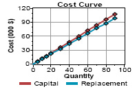 |
Figure 7 |
Converter
In this hybrid system, be sure to communicate between the consumer ac and the manufacturer dc is required to converter power electronics. Power converter is intended for system life expectancy of 15 years and 90% efficiency with a size of (10,15,20,30.40) is considered.
Diesel Generator
The cost of commercial diesel generators may250 kW / $ to 500 kW / $ change. The price per kW for smaller units rather than larger units. Free fuel prices 35 (L / $) is included. During the period of performance and value 0 and 35kW diesel 20000h to achieve optimal system is intended. The cost per kw about 450 $ and maintenance costs 400 $ for achieving optimal system are included. The curve shows the cost of diesel (IBM, 2011).
Optimization Results
Homer according to the inputs given to it. And the system may increase based on the final net cost of which in a table called Table Optimization is arranged. As the simulation is special arrangement of equipment modeling. Optimizing the best possible combination of through them is selected. The best combination is a combination that all of the constraints preset by the user to satisfied with minimal NPC. The optimization process homer all possible scenarios and impossible scenarios to simulate that cannot provide load request Eliminates. Then arrange them on the table and finally realized arrangement corresponds to the lowest npc as the optimum arrangement is introduced. depending on the price of fuel Various combinations are for the system based on the NPC to the city Bafgh and the time is shown in (Figure 10), shows that optimal system for Bafgh consists of solar array and diesel generator and battery.The results show that the optimal system includes solar array and diesel generator and battery is Bafgh city. The system is optimized for the city Bafgh including wind turbine and solar array and diesel generator .
 |
Figure 8 |
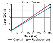 |
Figure 9 |
 |
Figure 10 |
Other states in figure11 shown by the software.
The results in terms of fuel prices for the city Bafgh shows the optimal system cost for delivering power to the city for 2017 need to invest (10821000) dollars. This article is in two parts, load forecasting and optimization of hybrid systems has been presented. The first was how to predict load and the results have been presented by software SPSS.These results indicate that once required Bafgh for the year 2017 is equal to 368,976 MWh (Centrell, 2012, IBM, 2011, Margeta, et al. 2012, Weersooriya, 1992).
 |
Figure 11 |
Conclusion
With regard to targeted subsidies, the results obtained for different part were varying. It was shown that consumption of agriculture sector was lower in the beginning of execution of the targeted subsidies. Moreover, after launching targeted subsidies, farmers decided to have electric wells because of higher price of fuel and consequently, effect of use of electric energy on load profile was obtained for 2017. Using electric wells has had adverse effect on agriculture sector. The results showed that Bafgh needs 368976 megawatt per hour in 2017.
With regard to low wind speed in Bafgh, optimal system was found to be solar-diesel and independent of network. Also, the results showed that with regard to high potential of Bafgh in wind and solar energies, Referring to[ Fig 11]government should invest in order to make use of the resources. The results obtained from optimization indicated that use of renewable energies increase if subsidies are completely removed so that diesel generators will decrease as fuel price increases. With regard to advantages of renewable plants in terms of environment, it is recommended to make use of such plants to reduce greenhouse gases.
The results indicate the necessity of governmental support in private sector in establishment of such systems. The recommended system in the present work can be the best solution for Bafgh in 2017.With regard to the results obtained from the present work, the following recommendations can be considered Modeling system in RETSCREEN Software in order to obtain reduction of greenhouse gases if the recommended system is adopted Determination of effect of using such systems on network parameters in connection to the system Use of other renewable resources in order to provide load and comparing the effect of costs and Modeling the systems by Homer Software.
References
- Arrillaga J., (1991), Computer Analysis of Power Systems, International energy agency.
- Centrell j., (2012), modeling the feasibility of using fuel cell and hydrogen internal combustion engines in remote renewable energy systems, National renewable energy laboratory.
- Chel A., Kaushik G., (2017), Renewable energy technologies for sustainable development of energy efficient building, Alexandria Engineering Journal, Available online, to be published.
- Chen H., (2000) Generation System Reliability Optimization, University of Saskatchewan.
- Elizabeth A., Anderson E., (1995), Judgmental and statistical methods of peak electric load management, International Journal of Forecasting, 11(2), 295-305
- Ghanbari A., Naghavi A., Ghaderi S. F., Sabaghian M., (2009), Artificial Neural Networks and regression approaches comparison for forecasting Iran’s annual electricity load, International Conference on Power Engineering, Energy and Electrical Drives, Lisbon,675-679.
- Hong Y. Y., Chang W. C., Chang T. R., Lee Y. D., Ouyang D. C, (2017), Optimal Sizing of Renewable Energy Generations in a Community Microgrid Using Markov Model, Energy, Available online, to be published.
- IBM, (2011), IBM SPSS Neural Networks 20 manual, Chicago.
- Jung J., Villaran M., (2017), Optimal planning and design of hybrid renewable energy systems for microgrids, Renewable and Sustainable Energy Reviews, 75, 180-191.
- Lakshminarasimman L. and Subramanian S., (2008), Applications of Differential Evolution in Power System Optimization, Advances in Differential Evolution, Volume 143 of the series Studies in Computational Intelligence, 257-273.
- Lippman A., (2004), Oil crises and climate challenges-30years of energy use in IEA countries, International energy agency.
- Mandal P., Senjyu T., Urasaki N., (2006), A Neural Network Based Several Hour Ahead Electric load Forecasting Using Similar Day Approach, International Journal of Electric Power and Energy System, 28(6), 367-373.
- Margeta J., Glasnovic Z., (2012) Theoretical settings of photovoltaic-hydro energy system for sustainable energy production, Solar Energy, 86(3), 972-982.
- Norusis M., (2011), IBM SPSS Statistics 19 Guide to Data Analysis.
- Passino K. M., (2002), Adaptive Pattern Recognition and Neural Network. Addison–Wesley Publishing Company, Int.
- Tezer T., Yaman R., Yaman G., (2017), Evaluation of approaches used for optimization of stand-alone hybrid renewable energy systems, Renewable and Sustainable Energy Reviews, 73, 840-853.
- Weersooriya, S., (1992), towards static security assessment of a large scale power system using neural networks, International energy agency.