Department of Mathematics, Maulana Azad National Institute of Technology Bhopal-462003, (M. P.) India
Article Publishing History
Received: 25/03/2018
Accepted After Revision: 10/06/2018
The paper deals with a model that describes a prey predator system with disease in the prey population where we have investigated the effect of harvest on the disease when vaccination strategies fail to recover the infected prey population. Many infectious diseases like varicella, which is a highly transferable infection caused by the varicella zoster virus and causes even death if untreated. When the disease affected the prey species, prey species is divided into two categories: susceptible prey and infected prey. From infected prey, the disease is transmitted to the susceptible prey species. It is assumed that infection effect both prey and predator species, but the disease is debilitating and ultimately causing death for predators. Once a predator is infected, it can be considered to be dead and infected prey does not recover due to failure of vaccination strategies. The infected prey species are subjected to harvesting at low and high harvesting rates. It is shown that effective harvesting of infected prey can control the spread of disease and prevent predator species from extinction. Equilibrium points are obtained by linearization and Jacobian matrix. The local and global stability of the various equilibrium points of the system was investigated. It is observed that coexistence of both the prey and predator species is possible through non-periodic solution due to the Bendixson-Dulac criterion. With the help of Routh-Hurwitz criterion and Liapunov function, local and global stability of the non-periodic orbits are determined. Some numerical simulations have been carried out to justify the results obtained.
Prey-Predator Model, Equilibrium Points, Stability Analysis, Harvesting Activity
Soni R, Chouhan U. A Dynamic Effect of Infectious Disease on Prey Predator System and Harvesting Policy. Biosc.Biotech.Res.Comm. 2018;11(2).
Soni R, Chouhan U. A Dynamic Effect of Infectious Disease on Prey Predator System and Harvesting Policy. Biosc.Biotech.Res.Comm. 2018;11(2). Available from: https://bit.ly/30ft5LE
Introduction
Mathematical models have become important tools in analyzing the dynamical relationship between predator and their prey. The predator prey system is one of the well-known models which have been studied and discussed a lot. The Lotka-Volterra predator prey system has been proposed to describe the population dynamics of two interacting species of a predator and its prey (Lotka, 1925, Volterra, 1931, Arb Von et al., 2013), Lotka–Volterra equation are of form
Where x and y are the prey and predator respectively; a is the growth rate of the prey (species) in the absence of interaction with the predator (species), b is the effect of the predation of species to species, c is the growth rate of species in perfect conditions: abundant prey and no negative environmental impact and d is the death rate of the species in perfect conditions: abundant prey and no negative environmental impact from natural cause. One of the unrealistic assumptions in the Lotka-Volterra model is that the growth of the prey populations is unbounded in the absence of the predator. Murray (Murray, 1989) modified the Lokta-Volterra model and the model were based on assumptions that the prey population exhibits logistic growth in the absence of predators, then the model obtained:
Materrial And Methods
We shall consider the following prey predator system for analyzing it mathematically,
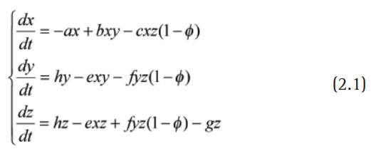
Where x, y and z stand for the density of susceptible predator, susceptible prey andinfected prey populations, respectively.And the parameters ‘a’ is the natural death of the healthy susceptible predator, ‘b’ is the number of contact between susceptible prey and healthy susceptible predator, ‘c’ is the number of contact between healthy susceptible predator and infected prey, ‘e’ is the number of contact between healthy susceptible predator with infected prey and susceptible prey, ‘f’ is the number of contact between healthy susceptible prey and infected prey, ‘g’ is the harvesting rate of infected prey , h is the per capita birth rate of susceptible prey (per time) and infected prey and ö is the proportion of those successively vaccinated at birth.
The model consists of basic assumptions that we have made in formulating the model are: The relative birth rate for infected prey and that of susceptible prey remains the same.The disease is severely weakened and ultimately causing death for the predators. Once a predator is infected, it can be assumed to be dead. We will therefore consider only susceptible predator andinfectious disease spreads among the prey population by contact, and the rate of infection is proportional to the infected and the susceptible prey.The predator makes no difference between susceptible and infected members of the prey population. The predator becomes infected by consuming the infected prey. The rate of predator infection is proportional to the product of infected prey and susceptible predators.The infected prey does not recover.
To begin with, let us find the equilibrium points of the system (2.1)
The system (2.1) has the following equilibrium points:
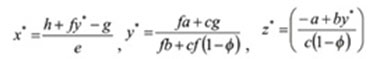
Where x*, y*, z* are given by
In the next section, let us discuss the stability of the five equilibrium points in the next which are obtained above.
Results and Discussion
Stability Analysis
In this section, we analyzed the local behavior of the system (2.1) around each equilibrium point. The Jacobian matrix of the system of state variables is as follows:
To determine the stability of the equilibrium points, we look at the most useful techniques for analyzing non-linear system is the linearized stability technique by theorem1.
Theorem 1:
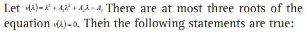
- If every root of the equation has absolute value less than one, then the equilibrium point of the system is locally asymptotically stable and equilibrium point is called a sink.
- If at-least one of the roots of the equation has an absolute value greater than one, then the equilibrium point of the system is unstable and equilibrium point is called a saddle.
- If every root of the equation has an absolute value greater than one, then the system is sourced.
- The equilibrium point of the system is called hyperbolic if no root of the equation has absolute value equal to one. If there exists a root of the equation with absolute value equal to one, then the equilibrium point is called non-hyperbolic (i.e. one eigenvalue has a vanishing real part).
Let us preparefour propositions in order to discuss the local stability around each equilibrium point.
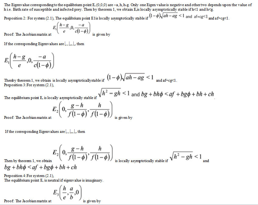
Preposition 1: For system (2.1),
The equilibrium point E0 is locally asymptotically stable if h<1 and h<g.
Proof: The Jacobian matrix at E0 (0,0,0) is given by
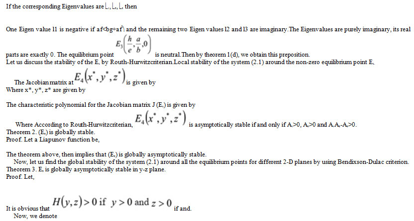
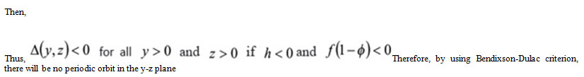
In the similar manner, we can show in the x-z plane for E1 with the condition ∆(x,z) < 0 for all x > 0 and z > 0 if h > 0, in the x-y plane for E3 with the condition ∆(x,z) < 0 for all x > 0 and y > 0 if h,b < 0 and in the same way E4 can be globally asymptotically stable in x-y,y-z and x-z planes.
We have performed some numerical simulation to study the role of harvesting on the prey predator system and we illustrate the dynamical and complex features of the model using MATLAB. In the starting, we fixed all parameters to ensure that the three classes of populations survive. Numerical simulations explain the effect of the parameters on the complex behavior of a given system (2.1).
(i) Let us consider following set of parameters,
a = 1.0; b = 1.5; c = 0.1; h = 0.5; e = 1.5;f=0.1;g=0.7,ö=0.91,
With initial condition x (0) =0. 8, y (0) =1. 70, z (0) =0. 75. For this set of parameter, we get the following variation of the population of the healthy predator, susceptible prey and infected prey with respect to time, which isillustrated below in figure 4 (a) and figure 4 (b).
(ii) Let us consider following set of parameters,
 |
Figure 4a: Represents the effect of high harvesting on the population of the infected prey as time goes on |
 |
Figure 4b: Represents the effect of high harvesting on the population of the healthy predator, susceptible prey and infected prey as time goes on. |
a = 1.0; b = 1.5; c = 0.1; h = 0.5; e = 1.5;f=0.1;g=0.1;ö=0.91;
With initial condition x (0) =0. 8, y (0) =1. 70, z (0) =0. 75. For this set of parameter, we get the following variation of the population of the healthy predator, susceptible prey and infected prey with respect to time, which is illustrated below in figure 4(c) and figure 4(d).
 |
Figure 4c: Represents the effect of low harvesting on the population of the infected prey as time goes on |
 |
Figure 4d: Represents the effect of low harvesting on the population of the healthy predator, susceptible prey and infected prey as time goes on |
It is observed that effective harvesting of diseased prey, increase the growth rate of the susceptible predator population. If the value of harvesting rate g≥0. 7 then the infected prey population decreases more rapidly, but if the value of g<0.7 then infected prey population decreases slowly that shown in fig. 4(a), 4(b), 4(c) and 4(d) respectively. In this analysis, we have also observed that the whole population of the susceptible predators may be wiped out due to increase in the number of the susceptible and infected preys. This result shows that the system is biologically well behaved. In another case when the diseased prey can be washed out, a rational use of the stability criterion of non-zero equilibrium point may be useful for ecological balance. In this case, the parameters of the system should be regulated in such a way that stability criterion of non-zero equilibrium is satisfied but infected prey remains low enough. Sometimes, harvesting became a suitable option for prevention of the population rather than the vaccination strategies. Therefore, effective harvesting became essential for the survival of the population.
Conclusion
A non-linear system based on the epidemic SIR model has been studied and discussed. Conditions for local and global stability at various equilibrium points were obtained. We have illustrated the effective harvesting of diseased prey in the whole system and reveal that the increases of predator population when the harvesting rate of infected prey population increases. We may conclude that effective harvesting of diseased prey may be used as a biological control for the spread of disease. And maintain balance in these species populations by preventing in the predator population to extinction. Finally, some numerical simulations illustrate and supplement our theoretical analysis by considering different parameter values. Low harvesting and high harvesting rates play an important role in this analysis. Global stability of equilibrium E0 shows that disease free equilibrium always exists. In future other effecting condition can be used to save the predator population by introducing alternative food for predator rather than diseased prey.
References
Arb Von and Rachel (2013), Predator Prey Models in Competitive Corporations,. Honors Program Projects, Paper 45.
Bakare E.A. et al. (2012), Mathematical Analysis of the Control of the Spread of Infectious Disease in a Prey-Predator Ecosystem, International Journal of Computer & Organization Trends –Volume 2 Issue 1.
Chattopadhyay J. and Arino O. (1999), A predator–prey model with disease in the prey, Nonlinear Analysis, Vol. 36, pp 747-766.
Das Krishna Pada (2014), Disease Control Through Harvesting – Conclusion drawn from a mathematical study of a Predator-Prey model with disease in both the population, International Journal of Biomathematics and Systems Biology, Volume 1, No. 1, pp 2394-7772.
E.A. Bakare Y.A Adekunle and A. Nwagwo (2012), Mathematical Analysis of the Control of the Spread of Infectious Disease in a Prey-Predator Ecosystem, International Journal of Computer & Organization Trends –Volume 2 Issue 1.
Herbert W.et al. (2000), The Mathematics of Infectious Diseases, SIAM Review, Vol. 42, No. 4., pp. 599-653.
Hethcote HW et al. (2004), A predator–prey model with infected prey, Theoretical Population Biology 66, pp 259–268.
Jia Yunfeng et al. (2017), Effect of predator cannibalism and prey growth on the dynamic behavior for a predator-stage structured population model with diffusion, J. Math. Anal. Appl., 449, 1479–1501.
Jia Yunfeng (2018), Analysis on dynamics of a population model with predator–prey-dependent functional response, Applied Mathematics Letters, Vol. 80, 64-70.
Johri Atul et al. (2012), Study of a Prey-Predator Model with Diseased Prey Int. J. Contemp. Math. Sciences,Vol. no. 10, 489–498.
Junej Nishant (2017), Effect of delay on globally stable prey–predator system, Chaos, Solitons & Fractals, Vol. 111, 146-156.
Sujatha et al. (2016), Dynamics in a Harvested Prey-Predator Model with Susceptible-Infected-Susceptible (SIS) Epidemic Disease in the Prey, Advances in Applied Mathematical Biosciences, Volume 7, Number 1, pp. 23-31.
Kapur J.K., Mathematical Models in Biology and Medicine, Published by Affiliated East-West Press Private Limited, pages-517.
Kermack W.O. and McKendrick A.G. (1927), A contribution to the mathematical theory of epidemics, Proc. R. Soc. Lond, 115, 700-721.
Kooi B.W., Venturino E. (2016), Ecoepidemic predator–prey model with feeding satiation, prey herd behavior and abandoned infected prey, Math. Biosci. 274, 58–72.
Lotka AJ. (1925), Elements of physical biology. Baltimore: Williams and Wilkins.
Mbava W. (2017) Prey, predator and super-predator model with disease in the super-predator, Applied Mathematics and Computation,Vol. 297, 92-114.
Murray J.D. (1989), Mathematical Biology, 2nd, Edition. Springer-Verlag, New York, 72-83.
Nandi Swapan Kumar and Mondal Prasanta Kumar (2015), Prey-Predator Model with Two-Stage Infection in Prey: Concerning Pest Control, Journal of Nonlinear Dynamics, Vol.15, 13 pages.
Pan Shuxia (2017), Invasion speed of a predator–prey system, Applied Mathematics Letters, Vol. 74, 46-51.
Singh Harkaran and Bhatti H.S. (2012), Stability of prey-predator model with harvesting activity of prey, International journal of pure and applied mathematics, volume 80 no. 5, 627-633.
Tang X. et al, (2015), Bifurcation analysis and turing instability in a diffusive predator-prey model with herd behavior and hyperbolic mortality, Chaos Solitons Fract. 81, 303–314.
Volterra V. (1931), Variations and fluctuations of a number of individuals in animal species living together, Newyork: McgrawHill, p. 409–48.
Yang Wenbin (2018), Analysis on existence of bifurcation solutions for a predator–prey model with herd behavior, Applied Mathematical Modelling, Vol. 53, 433-446.