
Environmental
Communication
Biosci. Biotech. Res. Comm. 10(1): 192-204 (2017)
Effect of barriers on the status of atmospheric
pollution by mathematical modelling
Zahra Naserzadeh
1
, Farideh Atabi
2
*, Faramarz Moattar
3
and Naser Moharram Nejad
4
1
Department of Environmental Engineering, Graduate School of Environment and Energy, Science and
Research Branch,Islamic Azad University, Tehran, Iran
2
Department of Environmental Engineering, Faculty of Environment and Energy, Science and Research
Branch,Islamic Azad University, Tehran, Iran
3
Department of Environmental Engineering, Faculty of Environment and Energy, Science and Research
Branch, Islamic Azad University, Tehran, Iran
4
Department of Environmental Engineering, Faculty of Environment and Energy, Science and Research
Branch, Islamic Azad University, Tehran, Iran
ABSTRACT
The prediction of material and gas polluting atmospheric distribution manner, is one of the important and propounded issues in indus-
tries especially oil, gas, petroleum and other similar industries. In recent years the world had witnessed a lot of environmental, hygienic
and security damages caused by the procedural events. So the prediction of the material diffusion, their consistency estimation according
to the environmental and atmospheric conditions, and the assessment of death rate caused by the polluters’ diffusion are the important
results of material atmospheric diffusion prediction. The required engineering and managing measures for confronting the probable
events can be performed by using these results. Two methods can be considered for prediction of polluters’ diffusion generally. The rst
method is utilized through using the real and experimental tests results and the eld measurement. In the second method some mod-
eling take place through different software such as HGSYSTEM, PHAST, ALOHA, SCREEN3, SLAB, CFX, and other prevalent polluter’s
diffusion modeling software that each one contains their own special competences and limitations. Among them the software such as
CFX which its calculations and modeling are based on the Computational Fluid Dynamics (CFD) method has got special importance for
high accuracy, 3D modeling, considering the obstacles in quality of diffusion, the competence of release modeling of materials which
are lighter and heavier than the air, and the ability in multi-phase compounds modeling (solid, liquid, gas). In this survey the Thorney
Island real experiment has been modeled through the aforesaid software for estimation of CFX amount of accuracy. The results show the
high CFX amount of accuracy with inconsiderable error in comparison to the real results of eld measurement of Thorney Island real
experiment. The output analytical results of CFX differ about 10 seconds with the experimental, real, and based on eld measurement
results. That means the rst gas densities in the desired point in analytical results has been sensed 10 seconds later.
KEY WORDS: THORNEY ISLAND, POLLUTERS’ DIFFUSION, CFX USING MODELING, CFD METHOD
192
ARTICLE INFORMATION:
*Corresponding Author: far-atabi@jamejam.net
Received 27
th
Nov, 2016
Accepted after revision 11
th
March, 2017
BBRC Print ISSN: 0974-6455
Online ISSN: 2321-4007
Thomson Reuters ISI ESC and Crossref Indexed Journal
NAAS Journal Score 2017: 4.31 Cosmos IF : 4.006
© A Society of Science and Nature Publication, 2017. All rights
reserved.
Online Contents Available at: http//www.bbrc.in/

Zahra Naserzadeh et al.
INTRODUCTION
Today the occurrence of environmental, hygienic and
security harsh events caused by the release, ignition, and
explosion of chemical and toxic materials in different
industrial units has necessitated the more than before
preparation for prevention or confrontation with these
dangers and accidents. So the places disposed the diffu-
sion and the dangerous material consistency are equal
or more than the fatal or dangerous materials there can
be recognized through prediction and material diffu-
sion quality modeling before the event occurrence and
reduce the amount of nancial, vital and environmental
damages through appropriate engineering and manag-
ing techniques in emergency conditions and crisis man-
agement plans at the time of event outbreak, (Siddiqui
et al. 2012).
In this regard, Yoshihito Tominaga proposed his
study, mentioned that Near- eld pollutant dispersion
in the urban environment involves the interaction of a
plume and the ow eld perturbed by building obsta-
cles. In the past two decades, micro-scale Computational
Fluid Dynamics (CFD) simulation of pollutant disper-
sion around buildings and in urban areas has been
widely used, sometimes in lieu of wind tunnel testing
(McBride et al. 2001). Key features of near- eld pollut-
ant dispersion around buildings from previous studies,
i.e., three-dimensionality of mean ow, unsteadiness
of large-scale ow structure, and anisotropy of tur-
bulent scalar uxes, are identi ed and discussed. It is
important to choose appropriate numerical models and
boundary conditions by understanding their inher-
ent strengths and limitations, (Sklavounos, and Rigas,
2004).
One of the rst studies in which CFD used to simu-
late emission of gases, the studies by Sutton et al.,(1986)
can be mentioned, that they used k- Turbulence model
to consider viscosity effects of turbulence. Using these
instruments faced with progress at computer hardware.
Perdikaris stated in this context that computational uid
dynamics (CFD) has been recognized as a potent tool for
realistic estimation of consequence of accidental loss of
containment because of its ability to take into account
the effect of complex terrain and obstacles present in
the path of dispersing uid (Gavelli, et al., 2008). In this
paper an attempt has been made to employ CFD in the
assessment of heavy gas dispersion in presence of obsta-
cles ( Hong-xi, et al., 2008).
Some workers have stated safety reports required for
sites storing quantities of dangerous substances in excess
of speci ed levels should include an assessment of the
risk associated with the facility, which will include an
evaluation of the effects of releases of dangerous sub-
stances to the environment. The models commonly used
for assessing the dispersion of dense gases in the atmos-
phere are based on the unobstructed terrain. They have
proposed physical modeling of releases in a Boundary
Layer Wind Tunnel (BLWT) and the use of Computa-
tional Fluid Dynamics (CFD).
These papers focus on the key ndings of the study,
which provide a dramatic insight into how terrain and
buildings can fundamentally alter the dispersion behav-
ior of dense gases. The results show how at terrain
models may overestimate the chlorine hazard range by
as much as a factor of 5, whilst the predicted direction of
travel of the cloud may err by up to 90 (Alberto and Hill,
2008). Kashi et al., (2009) in a study entitled “Tempera-
ture Gradient and Wind Pro le Effects on Heavy Gas
Dispersion in Build up Area”, stated dispersion of heavy
gases is considered to be more hazardous than the pas-
sive ones. This is because it takes place more slowly. In
this paper, based on the extensive experimental work of
Hanna and Chang, the CFD model was tested compared
with Kit Fox experiments. In order to accomplish this
validation, the multiphase approach was employed as
a new method in this area. In addition, the tempera-
ture gradient effects were investigated. The survey of
wind speed was done taking factors such as time, height
and direction into the consideration. To reduce the num-
ber of elements in computational domain, a combina-
tion of 2D and 3D geometries were utilized (Kashi, et al.
2009).
This paper deals with the evaluation of the atmos-
pheric dispersion CFD tool Fluid-PANACHE against
Prairie Grass and Kit Fox eld experiments. A descrip-
tion of the models for turbulence generation and dis-
sipation used (k–3 and k–l) and a comparison with the
Gaussian model ALOHA for both eld experiments are
also outlined, (Cormier et al. 2009).
As observed, many researchers provided a variety of
studies on accuracy of different turbulence models in
predicting emission. Study by Zhang et al. (2009) and
Gavllei in 2010 can be remembered here. Zhang has used
k- model to model gas emission with density over air.
The results of their study to the experimental results
found with acceptable error 2.2%. Currie et al. in 2012
using CFD examined how a heavy gas dispers in an
area and addressed evaluating risk regarding the results
(Zhang, 2009).
Given the progress in software and hardware contexts
particularly at the recent decade, using CFD to predict
how the pollutants emit at residential and industrial
areas has been increased. Indeed, CFD and/or modeling
ow in a three-dimensional form is as a virtual labora-
tory in which effect coming from different parameters
on ow can be examined easily with very low costs
rather than experimental methods like real measure-
ments, (Gavelli et al. 2010).
BIOSCIENCE BIOTECHNOLOGY RESEARCH COMMUNICATIONS THE EFFECT OF BARRIERS ON THE STATUS OF ATMOSPHERIC POLLUTION 193
Zahra Naserzadeh et al.
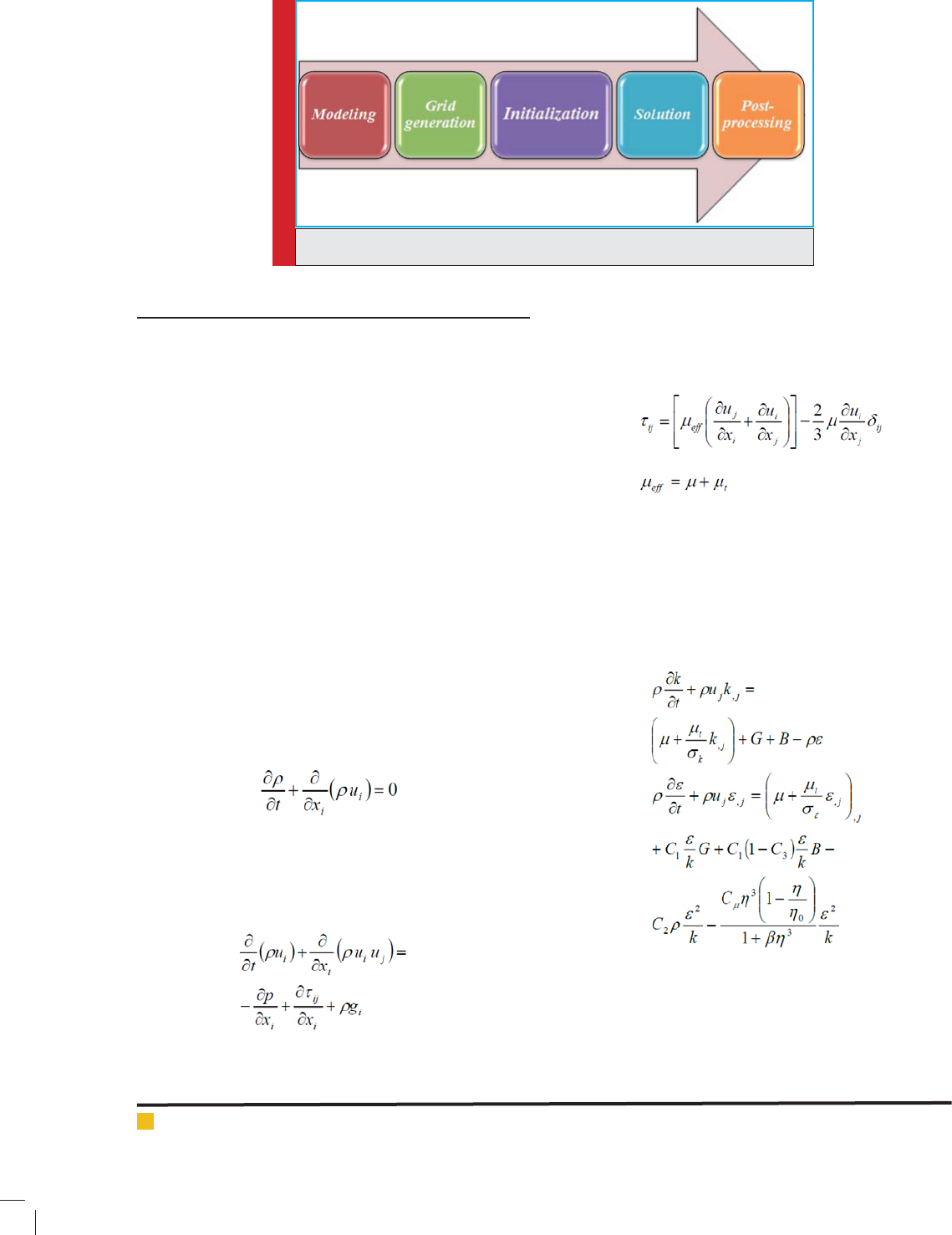
FIGURE 1. Total procedure for simulation process using CFD
MATERIALS AND METHODS
THREE-DIMENSIONAL SIMULATION ALGORITHM
To simulate using CFD, the speci c stages for simula-
tion process have to be paved and such stages dependent
from type and geometry are simulated, and they have
shown in gure 1.
One numerical method to resolve integral form of
prevailing equations is the Finite volume or the con-
trol volume. In this method, the physical amplitude is
divided to small volumes and the dependent variables
are measured at the center of volumes or in corners.
Equations resolving at the computational area regard-
ing the physical conditions of eld are the very Con-
servation equations of mass and momentum. Further, to
simulate disturbance of ow, transmission equations are
resolved for turbulence ow. This study aims to achieve
ammonia concentration at different times and places at
computational area. Thus, species conservation equation
has to be resolved at these problems. In following, a
summary of these equations has been addressed.
Species conservation equation is written as follows:
Where
and ui are uid density and components of
average speed.
The equation of motion extent and/or momentum at
direction i is written as follow:
In expression above, p,
ij
, pg
i
are Static pressure,
Stress tensor and Physical force of gravity in direction
of i. in expression 2, stress tensor is de ned as expres-
sion 3. In expression 3,
is molecular viscosity of the
uid and
is not of the features of uid, and is de ned
entitled Shear viscosity in turbulent ows.
Yakhot et al. proposed a new type of k- model in
which functional features and characteristics compared
to standard model reported. The proposed model based
on renormalized group theory reported so-called RNG.
RNG k- model in its physical form is similar to standard
model.
General form of equations at RNG k- is as follows:
In equation above, the additional term contains
parameter, indicating Characteristic time of turbulence
Characteristic time of the ow eld. Hence, model of
off-equilibrium effects have been also considered.
The main coef cients of model RNG for Isothermal
ows include:
,
k
, C
1
, C
2
, and C
. Two other coef -
(1)
(2)
(3)
(4)
194 THE EFFECT OF BARRIERS ON THE STATUS OF ATMOSPHERIC POLLUTION BIOSCIENCE BIOTECHNOLOGY RESEARCH COMMUNICATIONS
Zahra Naserzadeh et al.
cients, that is,
0
and using these coef cients and Von
Karman constant K are obtained. The coef cients below
are the ordinary coef cients used in this model.
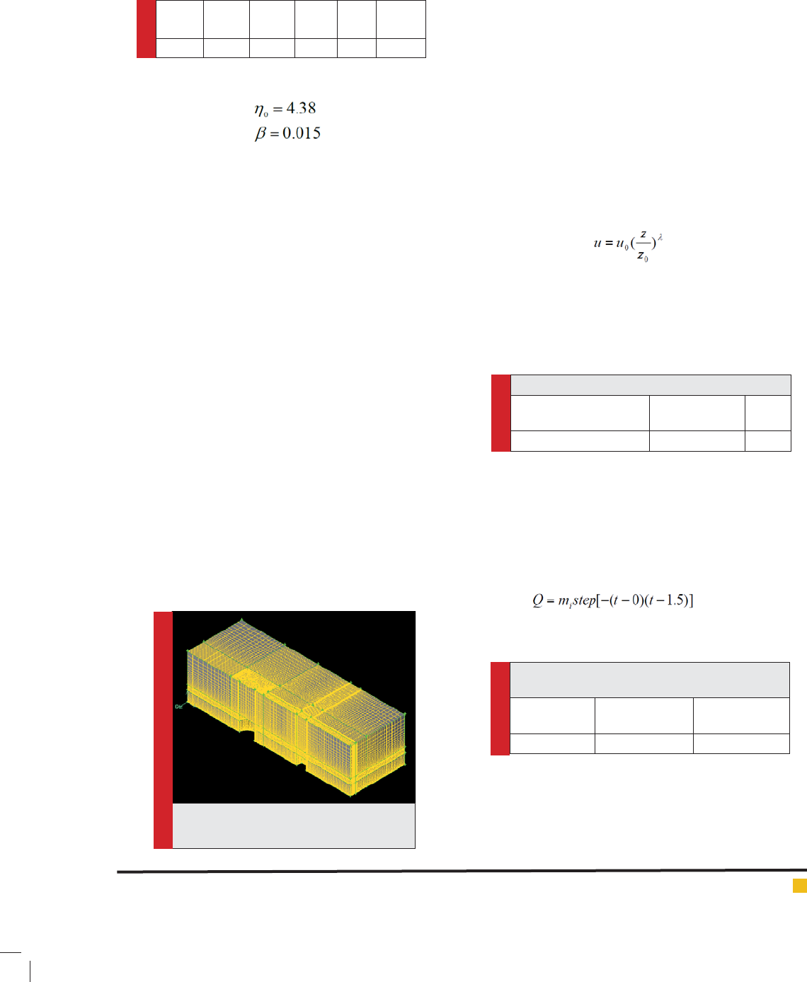
Geometry modeling and networking
Computational area in this modeling considered 150m
× 100m × 40m cube dimensions. Due to the geometry
and the symmetry with respect to the symmetry passing
through the center of the cube, the ow in symmetrical
regarding boundary conditions is solved. In gure 2, the
networking has been shown.
Applying boundary conditions
Wind input ow
Wind speed is one of the most important factors in the
spread and dilution of gas, and transmitted gas to differ-
ent parts of the range. If wind speed taken in a de ned
height, then the speed pro le using exponential expres-
sion can be expressed as follows:
Where is a dimensionless value and its value relies
on the extent of sustainability and also roughness of
dependant surface. Given the experiment conditions No
26, values of and roughness have been represented in
table 1 as shown below.
(6)
K
2
C
1
C
C
k
0.38751.681.420.0850.71790.7179
0
and are obtained using the coef cients below:
Modeling of Thorney Island real experiment through CFX
software based on CFD method:
In this study, the results of Thorney Island experiment
have been used for estimation of CFX amount of accu-
racy that computes and models based on CFD method.
The rst phase of eld experiments to spread heavy gas
dispersion trials at Thorney Island associated to release
of gas in an area without barrier considered, yet the sec-
ond phase of experiments aimed to examine heavier gas
dispersion than air in surrounding barriers.
In the experiments associated to a barrier, a cube 9m
× 9m × 9m, which was made of wood and plastic sheets
the trailers for moving obstacle and put it in the proper
position has been used; further, a trailer to displace bar-
rier and place it in proper positions have been used. Gas
supply cylinder (actually a 12-sided) with a diameter
of 14 meters and a height of 13 m, and a volume of
2000 cubic meters reported. In this part of the project of
Ammonia, Test Results for Project No. 26 Thorney Island
for assessment and veri cation of CFD has been used.
In this experiment, a cube barrier in distance placed 50
meter lower than cylinder. Ga mixture containing 68.4%
nitrogen and 31.6% Freon mentioned that during this
experiment, the wind speed has been measured approxi-
mately 1.9 m/s.
(5)
FIGURE 2. Networking computational eld
of Thorney Island
Table 1. features of wind pro le
Wind speed at the
reference height(m/s)
Roughness of
surface(m)
1.9 0.005 0.07
Gas input
According to the experiment no 26, about 2000 m
3
of gas mixture at lower than 1.5 second is released at
atmosphere to enter the boundary conditions at Tran-
sient state of mass ow rate, the gas mixture is de ned
through Step Function.
Where mi has been de ned in table 2.
(6)
Table 2. Values of mi, mass ow and the volume
of gas released
Total Released
Volume (m3)
Total Released
Mass (kg)
Mass In ow
Rate (kg/s)
197047673178
Walls
In the course of solving the steady state, barrier and
cylinder are taken into account, and in the course of
solving Transient state, barrier with the condition of the
BIOSCIENCE BIOTECHNOLOGY RESEARCH COMMUNICATIONS THE EFFECT OF BARRIERS ON THE STATUS OF ATMOSPHERIC POLLUTION 195
Zahra Naserzadeh et al.
walls is considered. Furthermore, the ground surface
is speci ed with the wall boundary condition. To the
earth surface, the roughness of surface with 0.005 meter,
and to the barrier and cylinder, the supposition of the
smooth surface is used.
Symmetry boundary condition
As mentioned, the plane of symmetry passing through
the center of the cube as the Symmetry boundary condi-
tion is considered. Furthermore, upper and lateral sur-
faces given that taken suf ciently far from barriers, and
the ow would sustain steady at this area, are de ned
with Symmetry boundary condition. In general, Sym-
metry boundary condition causes the gradient perpen-
dicular to the surface with different components at ow
eld taken equal to zero.
RESULTS AND DISCUSSION
The ow in nature in this problem taken as a transient
ow; to resolve transient ow, all the time considered
for modeling, time steps and early conditions have to
be taken as the input. To determine the early conditions,
in initial the ow has to be resolved in steady state and
its results have to be applied as the early conditions so
as to resolve the transient ow. In initial, the results of
stationary status were entered into discussion and later
the results associated to the transient ow have been
discussed as well.
The results of steady ow
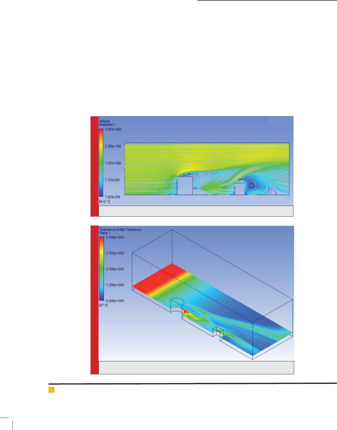
In gure 4, the ow lines in the plane of symmetry pass-
ing through the center at the computational area have
FIGURE 3. Flow lines for steady status
FIGURE 4. Eddie Frequency disturbance
196 THE EFFECT OF BARRIERS ON THE STATUS OF ATMOSPHERIC POLLUTION BIOSCIENCE BIOTECHNOLOGY RESEARCH COMMUNICATIONS
Zahra Naserzadeh et al.
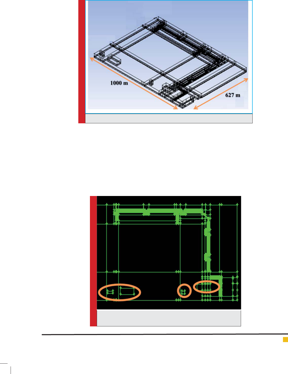
FIGURE 5. Dimensions of computational area
FIGURE 6. A perspective of the upward of geometry and position of
buildings
been shown. As expected, separation of ow and build-
ing Vortices behind the barriers can be seen. In gure 5,
Eddie Cantor frequency has been shown. As observed, at
most areas, this frequency placed at the area 1 Hz. As
a result, the time interval for Eddies at 1 second placed,
that this makes the comparison between experimental
results and numerical results possible.
Numerical analysis of ammonia leakage effect from
one of the ship tanks carrying ammonia in one of Iran’s
South Pars dock located in Asalooye area
This part of study aimed to provide numerical simu-
lation for ammonia leakage at one of Iran’s South Pars
dock located in Asalooye area. After ammonia produced
at Petrochemisty and distance about 1.5 km passed
through output Pipeline from petrochemical producers of
ammonia, this substance reaches to loading area at the
considered dock in a liquid form. This dock is particularly
for loading ethylene, butane, propane and ammonia. The
capacity of ships varied from 15 to 40 thousand tons.
Modern ships used today to prevent leakage are such two-
BIOSCIENCE BIOTECHNOLOGY RESEARCH COMMUNICATIONS THE EFFECT OF BARRIERS ON THE STATUS OF ATMOSPHERIC POLLUTION 197
Zahra Naserzadeh et al.
walledvessels. Also, a ship to be capable of carrying dif-
ferent types of liquid product or when damaged or leak to
any uids loaded to be lost, so such a ship is required to
be provided with different loading tanks.The ship under
study in this research contains 10 tanks. Since, possibil-
ity to damage to ships and leakage at them might come
to realize at least in one of the ship tanks, thus modeling
ammonia emission deriving from collapse of one ship
tank aimed in this project. In following, how to simulate
as well as the results have been proposed.
Geometric modeling and networking
According to the data given by Operations and Productiv-
ity, in average loading ships contain 10 tanks with 2000
m3, and as a result 10 Spherical tanks by diameter of
15.5 meter have been taken into consideration. The length
of ship has been taken 180 meter. In gure 9, dimensions
of computational area have been proposed. As observed,
this computational area includes different barriers in dif-
ferent forms. All the constituents existing in surrounding
dock have been modeled. The computational area includes
a series of Rack structures, pipelines transmission of pet-
rochemical products, two buildings beside each of docks,
the whole dock and administrative buildings.
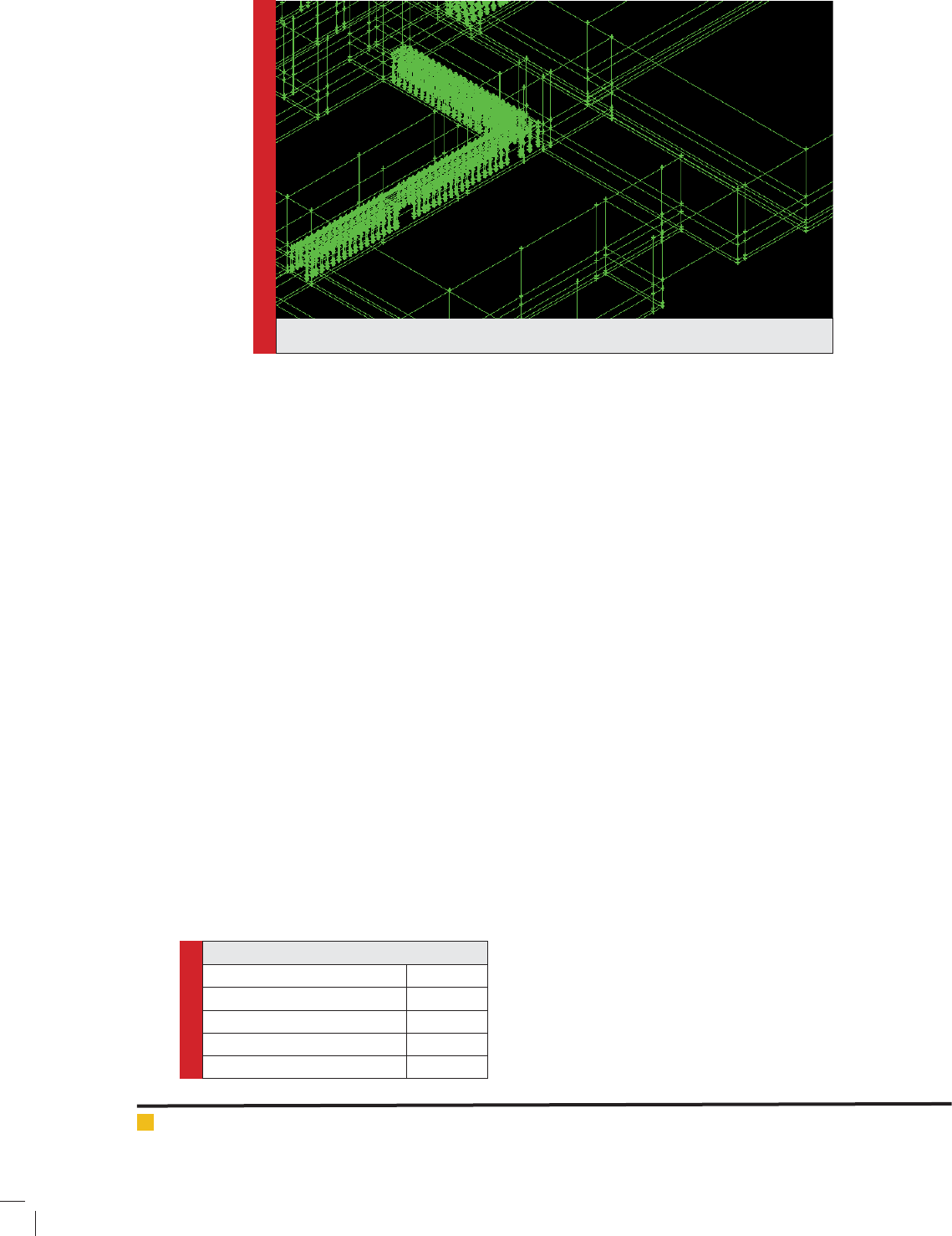
In gure 10, the upward perspective around dock, and
in gure 11, a part of geometry produced for Rack struc-
ture have been shown. In gure 10, areas speci ed with
orange color indicate administrative buildings. One of
the most optimal methods to reduce the elements used
simultaneously not the accuracy at results reduced, is the
very notion which lies in networking with organization.
In the complicated geometries, the only way to achieve
this aim is dividing the main geometry to smaller parts
with the capability of networking with organization in
them. For this, the computational area has been divided
into 456 pats with smaller volume.
These blocks can be observed in gure 11. Yet, accord-
ingly all the computational area cannot to be divided
into cubic blocks, so that the only way at the remained
areas would be the use of a disorganized network.
Yet in such an occasion, blocks in which disorgan-
ized network emerges are reduced; as a result, in a lower
space of computational area, disorganized network has
been produced. This can reduce the elements in a sub-
stantial amount. Finally, the number of networks pro-
duced would be 2893527.
Simulation using CFD
As mentioned, ship with 10 tanks mentioned with the
volume of 2000 m3. To model how the ammonia entered
to the area, all the ammonia existing in the tank has to
enter into area. For this, it is supposed the ammonia to
be entered to the area with Constant ow in a steady
status and in a little time. As a result regarding the com-
putations, it has been supposed that ammonia with ow
rate equal to 78667 kg/s for 15 seconds emits through
the surface of tank. The temperature of ammonia emit-
ted equals to -33 C0, that numerical modeling has been
carried out for 10 minutes. Further, the conditions of
area in autumn season at the studied area have been
FIGURE 7. the geometry produced for Rack structure
Table 3.
Temperature 30 C0
Wind speed 9.78 m/s
Sustainability class D
Flow angle relative to the Z axis 8 degree
Flow disturbance intensity 5%
198 THE EFFECT OF BARRIERS ON THE STATUS OF ATMOSPHERIC POLLUTION BIOSCIENCE BIOTECHNOLOGY RESEARCH COMMUNICATIONS
Zahra Naserzadeh et al.
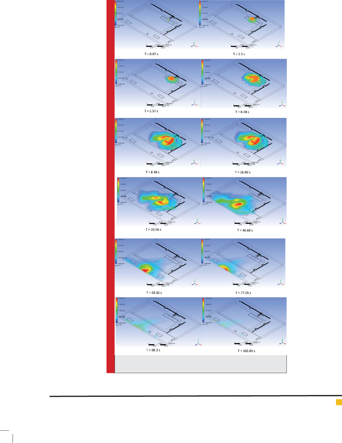
FIGURE 8. how ammonia emits at computational area at different time
intervals
BIOSCIENCE BIOTECHNOLOGY RESEARCH COMMUNICATIONS THE EFFECT OF BARRIERS ON THE STATUS OF ATMOSPHERIC POLLUTION 199
Zahra Naserzadeh et al.
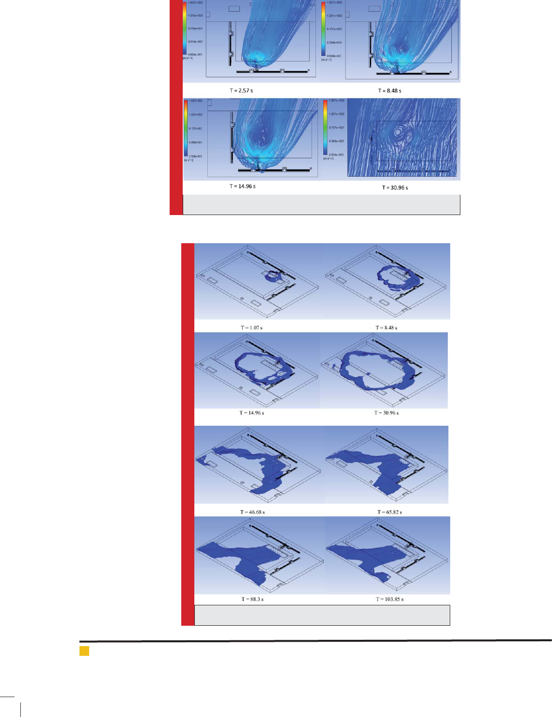
FIGURE 9. ow lines at different time intervals
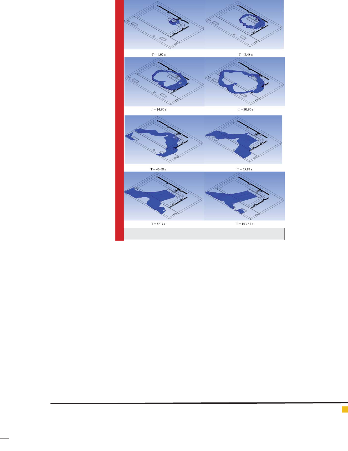
FIGURE 10. xed concentration surfaces 150 ppm de ning ERPG2
200 THE EFFECT OF BARRIERS ON THE STATUS OF ATMOSPHERIC POLLUTION BIOSCIENCE BIOTECHNOLOGY RESEARCH COMMUNICATIONS
Zahra Naserzadeh et al.
FIGURE 11. xed concentration surfaces 750 ppm de ning ERPG3
considered. The wind speed and temperature of environ-
ment have been taken 9.78 m/s and 30 C0, respectively.
APPLY BOUNDARY CONDITIONS
Wind ow input
According to the data associated to the meteorological
stations, wind speed has taken 9.8 m/s. in table 3, the
conditions acted for wind ow input have been regarded.
Wind ow output
At these surfaces, Pressure outlet boundary condition
has been used. The pressure regulated equals to 1 atmos-
pheric pressure.
Gas input
Here, a sudden collapse of ammonia tank might be faced.
As a result, to model sudden dispersion of ammonia,
supposed that all the mass existing in tank enter to the
computational area in a 15 seconds. As a result, it emits
with ow rate of 78667 kg/s. temperature of ammo-
nia emitted equals to -33 C
0
and Turbulence intensity
with 5%.
Symmetry boundary condition
Upward the computational area placed at a height in
which the gradient for ow parameters equals to zero.
As a result, the supposition to use symmetry boundary
condition at this surface is an acceptable supposition.
This condition considers the gradient perpendicular to
this surface for all the ow variables equaled to zero.
Wall boundary condition
All the solid surfaces at computational area like build-
ings, structures and pipes are de ned with Wall bound-
ary condition. This condition de nes the fact that the
gradient for the speed perpendicular to these surfaces is
equal to zero, or ow tangents to surfaces.
BIOSCIENCE BIOTECHNOLOGY RESEARCH COMMUNICATIONS THE EFFECT OF BARRIERS ON THE STATUS OF ATMOSPHERIC POLLUTION 201
Zahra Naserzadeh et al.
FIGURE 12. xed concentration surfaces 150 ppm de ning ERPG2
FIGURE 13. xed concentration surfaces 750 ppm de ning ERPG3
The regulations on how the convergence is
In the problems associated to transient ow, the early
conditions have to be determined in initial, that is,
resolving equations regarding time would be possible
only by determining the early condition. This is due to
the fact that the variables dependant to time are de ned
using the rst derivativetest. The early condition in the
given scenario is the parameters of eld before the pol-
lutants started to emit. As a result, the rst step is resolv-
ing the stationary ow to achieve the early conditions.
After the early conditions achieved, the eld parame-
ters over the time given speci ed time steps have to be
obtained. Determine time step to achieve more reliable
results is of importance. Select big time steps cause the
changes in the eld not to be achieved well, and not to
lead to reliable results. Small time steps cause substan-
tial computational cost comes to realize. The greatest
length that a particle has to pass from the center at ow
of the input surface to output surface equals to surface
diameter like the upward of computational eld, that
this diameter equals to 1180 meter. Assumed that this
particle passes the computational area with wind speed,
as a result passing time would be about 120 seconds.
Considering time step equals to 0.01 second, meant that
in case which particle moves from its position, a photo
taken of it for 12000 times, and/or in moving a particle
from eld the eld equations would be solved for 12000
times.
RESULTS
Firstly, how the ammonia emits at area has been pro-
posed in a three-dimensional way; gure 12 indicates it.
As observed, at the early seconds that ammonia with
a given ow rate enters to computational area, its emis-
sion would goes upward. By the passage of time, the
cloud formed moves in direction with wind. The most
important point in ammonia dispersion is its three-
dimensional behavior. As observed, ammonia expands
in line with z up to Rack structures. To understand bet-
ter how the concentration changes with time is, the ow
lines at different time intervals have been proposed. As
202 THE EFFECT OF BARRIERS ON THE STATUS OF ATMOSPHERIC POLLUTION BIOSCIENCE BIOTECHNOLOGY RESEARCH COMMUNICATIONS
Zahra Naserzadeh et al.
mentioned, to model sudden explosion of tank, sup-
posed that the whole mass existing in tank removes in
a short while. As a result, ammonia with a given ow
enters to the area from the tanks surfaces.
This means that ammonia from the surface of a sphere
with a given ow and speci c speed enters to the area.
This causes totally symmetric ow lines emerge at the
early times. Such ow lines remove from the tank per-
pendicular to it. This phenomenon at 2.57 second after
explosion can be observed in gure 13. The time takes
ammonia enters to area mentioned 15 seconds, and as a
result tank acts as a source till the early 15 seconds, yet
wind ow causes mass ow enters to the area in direc-
tion with wind. At 8.48 seconds after explosion, simulta-
neously removing ammonia from tank and moving pol-
lutants towards wind are observed. As pollutants move
towards wind, A rotating area has been built, and such a
rotating area and vortices that can be observed at 14.96
and 30.96 time intervals after the explosions, cause an
area with high ammonia concentration emerges at area.
This can be observed in gure 12.
Due to this vortex ow, the ammonia existing at this
area cannot remove from computational area with wind
speed. As a result, one leading factor that causes pol-
lutants concentration at area appears is the existence
of vortex ow. The most important limit to develop
response program at emergency conditions is the limit in
which effects of threatening individuals’ life exist. The
most important exposure limits used include:
- Emergency Response Planning Guideline (ERPG) belonged
to American Industrial Hygiene Association
- Immediately Dangerous to Life and Health (IDLH)
- Threshold Limit Values (TLV) belonged to American Con-
ference of Governmental Industrial Hygienists
ERPG exposure limit indicates the concentration that
causes effects on individuals’ health in compliance with
the existing concentrations seen.
ERPG1: This is the maximum airborne concentration
below which nearly all individuals could expose to the
substance as much as one hour, without any minor and
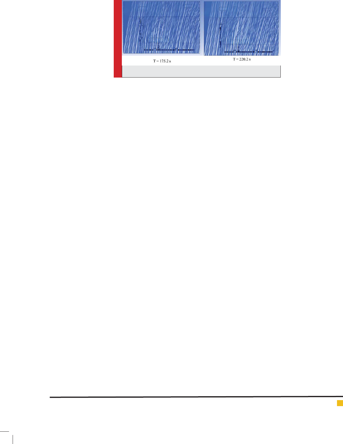
FIGURE 14. Flow lines at time intervals 175.2 and 220.2 seconds
temporary adverse effect on health imposed and smell
felt.
ERPG2: This is the maximum airborne concentration
below which nearly all individuals could be in this area
for an hour using protective instruments or measures.
ERPG3: This is the maximum airborne concentration
that causes mortality in exposure with the substance.
Values ERPG1, ERPG2 and ERPG3 for ammonia equal
to 25 ppm, 150 ppm and 750 pmm[20]. In gure 14 and
15, xed concentration levels including 150 ppm and
750 ppm indicating ERPG2 and ERPG3 have been pro-
posed. The rst point mentioned before is that pollutants
emission at the area is totally a three-dimensional phe-
nomenon, that this indicates the advantage of modeling
with CFD. The buildings at computational area include
two buildings to control docks located next to dock
inside water, as well as 5 buildings in land area .
These sectors include Chlorination unit, control tower,
power station, building services, parking lot. Based on
EPRG3 exposure limit followed by 30 seconds explo-
sion, the dock control center, control tower building
and electricity post are in uenced of ammonia pollut-
ant with 750 ppm concentration. followed by 65 sec-
onds after explosion, parking lot and service building
are also in uenced of this pollutant. Yet with regard to
the wind direction, the chlorination area is in uence of
this pollutant. The results about 2 minutes after explo-
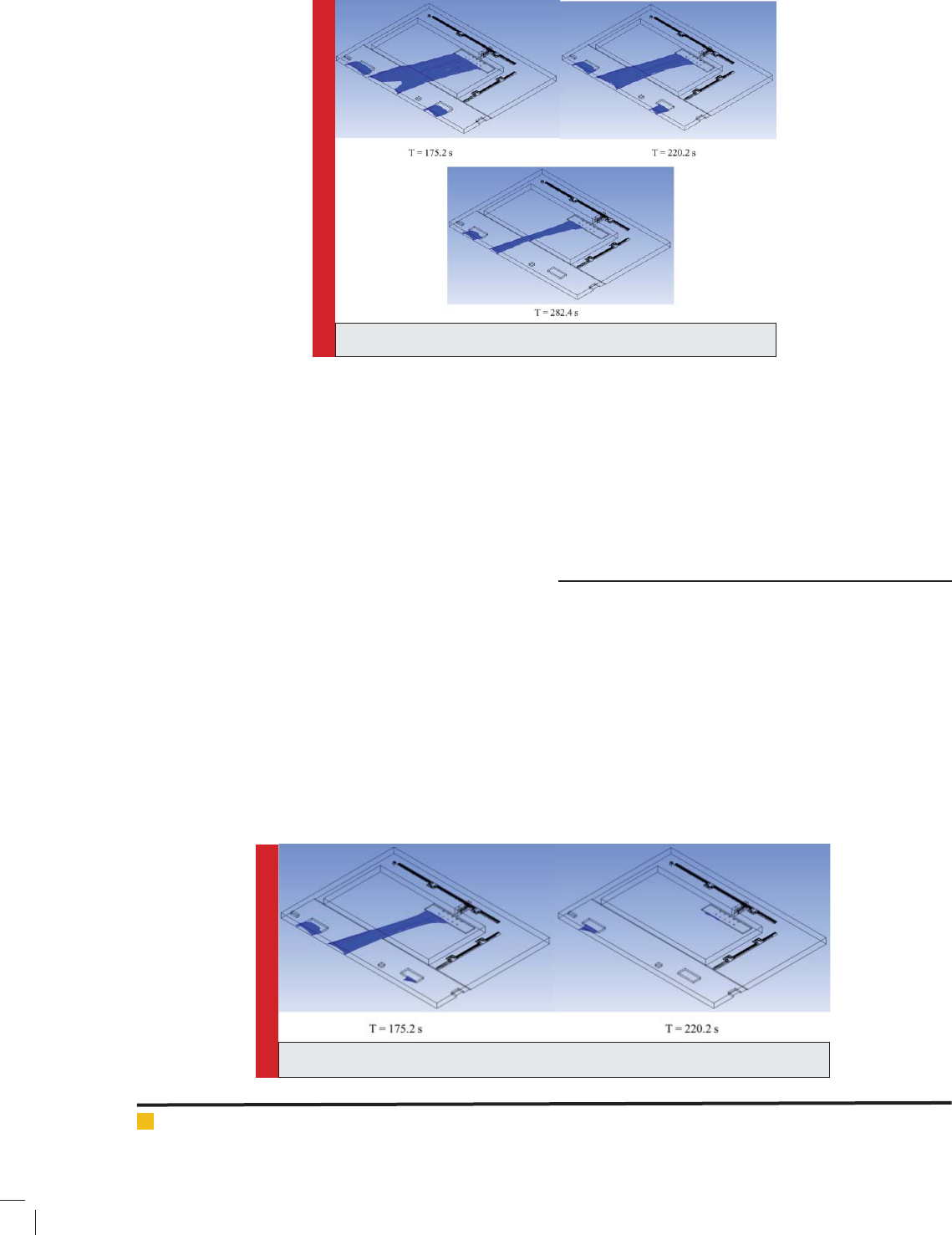
sion have been proposed in this part. In gure 16 and
17, ERPG2 and ERPG3 for different time intervals 175.2,
220.2 and 282.4 followed by emission have been shown.
By the passage of time, the limit in uenced of emission
reduces.
As de ned, pollutant accumulation at the areas where
vortex ow expected can be observed. This is due to
rotating and vortex ow. According to gure 17, the
most hazardous area in a sudden explosion in tank is
the area between service buildings and electricity post.
Further, due to rotating ow to 200 seconds followed by
emission, ammonia concentration with 750 ppm con-
centration behind the buildings located in land can be
observed. By the passage time and ammonia remove
BIOSCIENCE BIOTECHNOLOGY RESEARCH COMMUNICATIONS THE EFFECT OF BARRIERS ON THE STATUS OF ATMOSPHERIC POLLUTION 203
Zahra Naserzadeh et al.
from the computational area modeled in this study,
ammonia enters to the petrochemicals upward the dock.
Due to wind ow direction, two petrochemicals would
be in uenced of ammonia dispersion. Further, the xed
concentration levels at 282.4 second followed by emis-
sion have not been proposed in gure 17. The reason
for this lies in removing pollutant from computational
area, that a surface with xed concentration 750 ppm
does not exist at this time interval. Finally, ow lines
have been proposed at this time interval. As speci ed,
the ow eld found stationary after 4 minutes.
SUGGESTIONS
According to the results of the research the software
such as CFX that computes and models based on CFD
method, with inconsiderable error, are appropriate and
reliable for modeling of gas polluter diffusion in the
atmosphere, therefore the use of these software instead
of Gaussian equation based one is highly recommended.
REFERENCES
Alberto, M. and Hill, T. (2008) CFD and Gaussian atmospheric
dispersion models: A comparison for leak from carbon dioxide
transportation and storage facilities. Atmospheric Environ-
ment, 2008.
Cormier, B. R., Qi, R., Yun, G., Zhang, Y., & Sam Mannan, M.
(2009) Application of computational uid dynamics for LNG
vapor dispersion modeling: a study of key parameters. Journal
of Loss Prevention in the Process Industries, 2009.
Kashi, E., et al.(2009) Effects of Vertical Temperature Gradient
on Heavy Gas Dispersion in Build up Area. Iranian Journal of
Chemical Engineering, 2009.
Gavelli, F, Bullister, E. and Kytomaa, H. (2008)Application of
CFD (Fluent) to LNG spills into geometrically complex envi-
ronments. Journal of Hazardous Materials, 2008.
Gavelli, F., Chernovsky, M. K., Bullister, E., & Kytomaa, H. K.
(2010) Modeling of LNG spills into trenches. Journal of Haz-
ardous Materials, 2010.
McBride, M. A., Reeves, A. B., Vanderheyden, M. D., Lea, C.
J., & Zhou, X.(2001) Use of advanced techniques to model the
dispersion of chlorine in complex terrain. Process Safety and
Environmental Protection, 2001.
Siddiqui, M., Jayanti, S. and Swaminathan, T.(2012) CFD anal-
ysis of dense gas dispersion in indoor environment for risk
assessment and risk mitigation. Journal of Hazardous Materi-
als, 2012.
Sklavounos, S. and Rigas, F.(2004) Validation of turbulence
models in heavy gas dispersion over obstacles. Journal of Haz-
ardous Materials, 2004.
Tominaga, Y. and Stathopoulos, T. (2013)CFD simulation of
near- eld pollutant dispersion in the urban environment: A
review of current modeling techniques.Atmospheric Environ-
ment, 2013.
YU Hong-xi, et al., (2008) Numerical simulation of leakage and
dispersion of acid gas in gathering pipeline. Journal of China
University of Petroleum, 2008.
Zhang, C. N., Ning, P., & Ma, C. X.(2009) Numerical simulation
of dense gas leakage in plateau city at complex terrain. Journal
of Wuhan University of Technology, 2009.
204 THE EFFECT OF BARRIERS ON THE STATUS OF ATMOSPHERIC POLLUTION BIOSCIENCE BIOTECHNOLOGY RESEARCH COMMUNICATIONS